这一页开头是 6 份课件的 公式总表 ,后面按 exam Practice 的 7 道题整理成 5 个知识点。每个知识点先列核心公式,再放考试题,最后放课件(Lecture)和作业(HW)里对应的例题。点击 查看答案 展开解答。
0. 公式总表(Lecture 01–06)
按课件顺序整理,括号里是课件页码。考试前从头到尾过一遍。
Lecture 01 · 概率与统计复习
常见分布
分布 PMF / PDF E ( X ) E(X) E ( X ) Var ( X ) \operatorname{Var}(X) Var ( X ) Bernoulli( p ) (p) ( p ) p ( x ) = p x ( 1 − p ) 1 − x , x ∈ { 0 , 1 } p(x)=p^x(1-p)^{1-x},\ x\in\{0,1\} p ( x ) = p x ( 1 − p ) 1 − x , x ∈ { 0 , 1 } p p p p ( 1 − p ) p(1-p) p ( 1 − p ) Binomial( n , p ) (n,p) ( n , p ) ( n x ) p x ( 1 − p ) n − x \binom{n}{x}p^x(1-p)^{n-x} ( x n ) p x ( 1 − p ) n − x n p np n p n p ( 1 − p ) np(1-p) n p ( 1 − p ) Poisson( λ ) (\lambda) ( λ ) e − λ λ x x ! \dfrac{e^{-\lambda}\lambda^x}{x!} x ! e − λ λ x λ \lambda λ λ \lambda λ Normal( μ , σ 2 ) (\mu,\sigma^2) ( μ , σ 2 ) 1 σ 2 π exp [ − ( x − μ ) 2 2 σ 2 ] \dfrac{1}{\sigma\sqrt{2\pi}}\exp\!\Big[-\dfrac{(x-\mu)^2}{2\sigma^2}\Big] σ 2 π 1 exp [ − 2 σ 2 ( x − μ ) 2 ] μ \mu μ σ 2 \sigma^2 σ 2
Poisson 过程 (p.59):P ( N ( t ) = n ) = ( λ t ) n e − λ t n ! P(N(t)=n)=\dfrac{(\lambda t)^ne^{-\lambda t}}{n!} P ( N ( t ) = n ) = n ! ( λ t ) n e − λ t E [ N ( t ) ] = λ t E[N(t)]=\lambda t E [ N ( t )] = λ t
标准化 (p.66, 86):Z = X − μ σ ∼ N ( 0 , 1 ) Z=\dfrac{X-\mu}{\sigma}\sim N(0,1) Z = σ X − μ ∼ N ( 0 , 1 ) Φ ( t ) = P ( Z < t ) \Phi(t)=P(Z<t) Φ ( t ) = P ( Z < t )
条件概率与 Bayes 公式 (p.70–71)
P ( A ∣ B ) = P ( A B ) P ( B ) , P ( B ∣ A ) = P ( A ∣ B ) P ( B ) P ( A ) , P ( A ) = ∑ i P ( A ∣ B i ) P ( B i ) P(A\mid B)=\frac{P(AB)}{P(B)},\qquad P(B\mid A)=\frac{P(A\mid B)P(B)}{P(A)},\qquad P(A)=\sum_iP(A\mid B_i)P(B_i) P ( A ∣ B ) = P ( B ) P ( A B ) , P ( B ∣ A ) = P ( A ) P ( A ∣ B ) P ( B ) , P ( A ) = i ∑ P ( A ∣ B i ) P ( B i ) 期望与方差 (p.76–84)
E ( X ) = ∑ x x p ( x ) 或 ∫ − ∞ ∞ x f ( x ) d x , Var ( X ) = E [ ( X − μ ) 2 ] = E ( X 2 ) − [ E ( X ) ] 2 E(X)=\sum_x x\,p(x)\ \ \text{或}\ \ \int_{-\infty}^{\infty}x f(x)\,dx,\qquad \operatorname{Var}(X)=E[(X-\mu)^2]=E(X^2)-[E(X)]^2 E ( X ) = x ∑ x p ( x ) 或 ∫ − ∞ ∞ x f ( x ) d x , Var ( X ) = E [( X − μ ) 2 ] = E ( X 2 ) − [ E ( X ) ] 2 E ( a X + b ) = a E ( X ) + b , Var ( a X + b ) = a 2 Var ( X ) , σ a X + b = ∣ a ∣ σ X E(aX+b)=aE(X)+b,\qquad \operatorname{Var}(aX+b)=a^2\operatorname{Var}(X),\qquad \sigma_{aX+b}=|a|\sigma_X E ( a X + b ) = a E ( X ) + b , Var ( a X + b ) = a 2 Var ( X ) , σ a X + b = ∣ a ∣ σ X 协方差与相关系数 (p.85)
Cov ( X , Y ) = E [ ( X − μ X ) ( Y − μ Y ) ] , ρ = σ X Y σ X σ Y ∈ [ − 1 , 1 ] \operatorname{Cov}(X,Y)=E[(X-\mu_X)(Y-\mu_Y)],\qquad \rho=\frac{\sigma_{XY}}{\sigma_X\sigma_Y}\in[-1,1] Cov ( X , Y ) = E [( X − μ X ) ( Y − μ Y )] , ρ = σ X σ Y σ X Y ∈ [ − 1 , 1 ] Var ( X ± Y ) = Var ( X ) + Var ( Y ) ± 2 Cov ( X , Y ) \operatorname{Var}(X\pm Y)=\operatorname{Var}(X)+\operatorname{Var}(Y)\pm2\operatorname{Cov}(X,Y) Var ( X ± Y ) = Var ( X ) + Var ( Y ) ± 2 Cov ( X , Y ) 独立 ⇒ Cov = 0 \operatorname{Cov}=0 Cov = 0
Lecture 02 · 预测建模基础
模型与误差分解 (p.17, 44)
Y = f ( X ) + ε , E [ ( Y − Y ^ ) 2 ] = [ f ( X ) − f ^ ( X ) ] 2 ⏟ reducible + Var ( ε ) ⏟ irreducible Y=f(X)+\varepsilon,\qquad E\big[(Y-\hat Y)^2\big]=\underbrace{[f(X)-\hat f(X)]^2}_{\text{reducible}}+\underbrace{\operatorname{Var}(\varepsilon)}_{\text{irreducible}} Y = f ( X ) + ε , E [ ( Y − Y ^ ) 2 ] = reducible [ f ( X ) − f ^ ( X ) ] 2 + irreducible Var ( ε ) MSE 与偏差-方差分解 (p.34, 42–44)
M S E = 1 n ∑ i = 1 n ( y i − f ^ ( x i ) ) 2 , E [ ( y 0 − f ^ ( x 0 ) ) 2 ] = Var ( f ^ ( x 0 ) ) + [ Bias ( f ^ ( x 0 ) ) ] 2 + Var ( ε ) MSE=\frac1n\sum_{i=1}^n\big(y_i-\hat f(x_i)\big)^2,\qquad E\big[(y_0-\hat f(x_0))^2\big]=\operatorname{Var}(\hat f(x_0))+[\operatorname{Bias}(\hat f(x_0))]^2+\operatorname{Var}(\varepsilon) M S E = n 1 i = 1 ∑ n ( y i − f ^ ( x i ) ) 2 , E [ ( y 0 − f ^ ( x 0 ) ) 2 ] = Var ( f ^ ( x 0 )) + [ Bias ( f ^ ( x 0 )) ] 2 + Var ( ε ) 无偏估计量 (p.40–41)
定义:E ( Θ ^ ) = θ E(\hat\Theta)=\theta E ( Θ ^ ) = θ Bias = E ( Θ ^ ) − θ \operatorname{Bias}=E(\hat\Theta)-\theta Bias = E ( Θ ^ ) − θ
样本均值无偏:X ˉ = 1 n ∑ X i \bar X=\dfrac1n\sum X_i X ˉ = n 1 ∑ X i E ( X ˉ ) = μ E(\bar X)=\mu E ( X ˉ ) = μ Var ( X ˉ ) = σ 2 n \operatorname{Var}(\bar X)=\dfrac{\sigma^2}{n} Var ( X ˉ ) = n σ 2
样本方差无偏(分母是 n − 1 n-1 n − 1 :
S 2 = 1 n − 1 ∑ i = 1 n ( X i − X ˉ ) 2 , E ( S 2 ) = σ 2 S^2=\frac{1}{n-1}\sum_{i=1}^n(X_i-\bar X)^2,\qquad E(S^2)=\sigma^2 S 2 = n − 1 1 i = 1 ∑ n ( X i − X ˉ ) 2 , E ( S 2 ) = σ 2 证明要点:E [ ∑ ( X i − X ˉ ) 2 ] = ∑ E ( X i 2 ) − n E ( X ˉ 2 ) = n ( σ 2 + μ 2 ) − n ( σ 2 n + μ 2 ) = ( n − 1 ) σ 2 E\big[\sum(X_i-\bar X)^2\big]=\sum E(X_i^2)-nE(\bar X^2)=n(\sigma^2+\mu^2)-n\big(\tfrac{\sigma^2}{n}+\mu^2\big)=(n-1)\sigma^2 E [ ∑ ( X i − X ˉ ) 2 ] = ∑ E ( X i 2 ) − n E ( X ˉ 2 ) = n ( σ 2 + μ 2 ) − n ( n σ 2 + μ 2 ) = ( n − 1 ) σ 2
在所有无偏估计量中方差最小的叫 minimum variance unbiased estimator (MVUE) 。
分类误差、Bayes 分类器与 KNN (p.46–49)
Error rate = 1 n ∑ i = 1 n I ( y i ≠ y ^ i ) , Bayes: y ^ 0 = arg max j Pr ( Y = j ∣ X = x 0 ) \text{Error rate}=\frac1n\sum_{i=1}^nI(y_i\ne\hat y_i),\qquad \text{Bayes: }\hat y_0=\arg\max_j\Pr(Y=j\mid X=x_0) Error rate = n 1 i = 1 ∑ n I ( y i = y ^ i ) , Bayes: y ^ 0 = arg j max Pr ( Y = j ∣ X = x 0 ) Bayes error rate = 1 − E [ max j Pr ( Y = j ∣ X ) ] , KNN: Pr ( Y = j ∣ X = x 0 ) = 1 K ∑ i ∈ N 0 I ( y i = j ) \text{Bayes error rate}=1-E\Big[\max_j\Pr(Y=j\mid X)\Big],\qquad \text{KNN: }\Pr(Y=j\mid X=x_0)=\frac1K\sum_{i\in N_0}I(y_i=j) Bayes error rate = 1 − E [ j max Pr ( Y = j ∣ X ) ] , KNN: Pr ( Y = j ∣ X = x 0 ) = K 1 i ∈ N 0 ∑ I ( y i = j ) Lecture 03 · 简单线性回归
模型与最小二乘 (p.8–9)
Y = β 0 + β 1 x + ε , S x x = ∑ ( x i − x ˉ ) 2 = ∑ x i 2 − ( ∑ x i ) 2 n , S x y = ∑ ( x i − x ˉ ) ( y i − y ˉ ) = ∑ x i y i − ( ∑ x i ) ( ∑ y i ) n Y=\beta_0+\beta_1x+\varepsilon,\qquad S_{xx}=\sum(x_i-\bar x)^2=\sum x_i^2-\frac{(\sum x_i)^2}{n},\qquad S_{xy}=\sum(x_i-\bar x)(y_i-\bar y)=\sum x_iy_i-\frac{(\sum x_i)(\sum y_i)}{n} Y = β 0 + β 1 x + ε , S xx = ∑ ( x i − x ˉ ) 2 = ∑ x i 2 − n ( ∑ x i ) 2 , S x y = ∑ ( x i − x ˉ ) ( y i − y ˉ ) = ∑ x i y i − n ( ∑ x i ) ( ∑ y i ) β ^ 1 = S x y S x x , β ^ 0 = y ˉ − β ^ 1 x ˉ , e i = y i − y ^ i \hat\beta_1=\frac{S_{xy}}{S_{xx}},\qquad \hat\beta_0=\bar y-\hat\beta_1\bar x,\qquad e_i=y_i-\hat y_i β ^ 1 = S xx S x y , β ^ 0 = y ˉ − β ^ 1 x ˉ , e i = y i − y ^ i σ 2 \sigma^2 σ 2
S S E = ∑ i = 1 n ( y i − y ^ i ) 2 , σ ^ 2 = S S E n − 2 SS_E=\sum_{i=1}^n(y_i-\hat y_i)^2,\qquad \hat\sigma^2=\frac{SS_E}{n-2} S S E = i = 1 ∑ n ( y i − y ^ i ) 2 , σ ^ 2 = n − 2 S S E (分母 n − 2 n-2 n − 2 β 0 , β 1 \beta_0,\beta_1 β 0 , β 1 n − p n-p n − p
系数的期望、方差与标准误 (p.16)
E ( β ^ 1 ) = β 1 , V ( β ^ 1 ) = σ 2 S x x , E ( β ^ 0 ) = β 0 , V ( β ^ 0 ) = σ 2 [ 1 n + x ˉ 2 S x x ] E(\hat\beta_1)=\beta_1,\quad V(\hat\beta_1)=\frac{\sigma^2}{S_{xx}},\qquad E(\hat\beta_0)=\beta_0,\quad V(\hat\beta_0)=\sigma^2\Big[\frac1n+\frac{\bar x^2}{S_{xx}}\Big] E ( β ^ 1 ) = β 1 , V ( β ^ 1 ) = S xx σ 2 , E ( β ^ 0 ) = β 0 , V ( β ^ 0 ) = σ 2 [ n 1 + S xx x ˉ 2 ] s e ( β ^ 1 ) = σ ^ 2 S x x , s e ( β ^ 0 ) = σ ^ 2 [ 1 n + x ˉ 2 S x x ] se(\hat\beta_1)=\sqrt{\frac{\hat\sigma^2}{S_{xx}}},\qquad se(\hat\beta_0)=\sqrt{\hat\sigma^2\Big[\frac1n+\frac{\bar x^2}{S_{xx}}\Big]} se ( β ^ 1 ) = S xx σ ^ 2 , se ( β ^ 0 ) = σ ^ 2 [ n 1 + S xx x ˉ 2 ] t 检验与置信区间 (p.13–20)
T = X ˉ − μ S / n ∼ t n − 1 , X ˉ ± t α / 2 , n − 1 S n T=\frac{\bar X-\mu}{S/\sqrt n}\sim t_{n-1},\qquad \bar X\pm t_{\alpha/2,n-1}\frac{S}{\sqrt n} T = S / n X ˉ − μ ∼ t n − 1 , X ˉ ± t α /2 , n − 1 n S T 0 = β ^ 1 − β 1 , 0 s e ( β ^ 1 ) ∼ t n − 2 , β ^ 1 ± t α / 2 , n − 2 σ ^ 2 S x x , β ^ 0 ± t α / 2 , n − 2 σ ^ 2 [ 1 n + x ˉ 2 S x x ] T_0=\frac{\hat\beta_1-\beta_{1,0}}{se(\hat\beta_1)}\sim t_{n-2},\qquad \hat\beta_1\pm t_{\alpha/2,n-2}\sqrt{\frac{\hat\sigma^2}{S_{xx}}},\qquad \hat\beta_0\pm t_{\alpha/2,n-2}\sqrt{\hat\sigma^2\Big[\frac1n+\frac{\bar x^2}{S_{xx}}\Big]} T 0 = se ( β ^ 1 ) β ^ 1 − β 1 , 0 ∼ t n − 2 , β ^ 1 ± t α /2 , n − 2 S xx σ ^ 2 , β ^ 0 ± t α /2 , n − 2 σ ^ 2 [ n 1 + S xx x ˉ 2 ] 预测区间 (p.23–24)
y ^ 0 ± t α / 2 , n − 2 σ ^ 2 [ 1 + 1 n + ( x 0 − x ˉ ) 2 S x x ] \hat y_0\pm t_{\alpha/2,n-2}\sqrt{\hat\sigma^2\Big[1+\frac1n+\frac{(x_0-\bar x)^2}{S_{xx}}\Big]} y ^ 0 ± t α /2 , n − 2 σ ^ 2 [ 1 + n 1 + S xx ( x 0 − x ˉ ) 2 ] 预测区间永远比均值置信区间宽,多出的“1”来自新观测本身的误差。
ANOVA (p.25)
S S T = ∑ ( y i − y ˉ ) 2 = S S R + S S E , S S R = ∑ ( y ^ i − y ˉ ) 2 SS_T=\sum(y_i-\bar y)^2=SS_R+SS_E,\qquad SS_R=\sum(\hat y_i-\bar y)^2 S S T = ∑ ( y i − y ˉ ) 2 = S S R + S S E , S S R = ∑ ( y ^ i − y ˉ ) 2 相关系数与回归 (p.29)
ρ = σ X Y σ X σ Y , β 1 = ρ σ Y σ X , β 0 = μ Y − μ X ρ σ Y σ X \rho=\frac{\sigma_{XY}}{\sigma_X\sigma_Y},\qquad \beta_1=\rho\frac{\sigma_Y}{\sigma_X},\qquad \beta_0=\mu_Y-\mu_X\rho\frac{\sigma_Y}{\sigma_X} ρ = σ X σ Y σ X Y , β 1 = ρ σ X σ Y , β 0 = μ Y − μ X ρ σ X σ Y 最大似然 (p.35–38)
L ( θ ) = ∏ i = 1 n f ( x i ∣ θ ) , l ( β 0 , β 1 , σ 2 ) = − n 2 ln 2 π − n 2 ln σ 2 − 1 2 σ 2 ∑ ( y i − β 0 − β 1 x i ) 2 L(\theta)=\prod_{i=1}^nf(x_i\mid\theta),\qquad l(\beta_0,\beta_1,\sigma^2)=-\frac n2\ln2\pi-\frac n2\ln\sigma^2-\frac{1}{2\sigma^2}\sum(y_i-\beta_0-\beta_1x_i)^2 L ( θ ) = i = 1 ∏ n f ( x i ∣ θ ) , l ( β 0 , β 1 , σ 2 ) = − 2 n ln 2 π − 2 n ln σ 2 − 2 σ 2 1 ∑ ( y i − β 0 − β 1 x i ) 2 对 β 0 , β 1 \beta_0,\beta_1 β 0 , β 1 σ 2 \sigma^2 σ 2 S S E n \dfrac{SS_E}{n} n S S E S S E n − 2 \dfrac{SS_E}{n-2} n − 2 S S E
Lecture 04 · 多元线性回归
模型与矩阵形式 (p.6, 14–15)
y i = β 0 + ∑ j = 1 k β j x i j + ε i , y = X β + ε , β ^ = ( X ′ X ) − 1 X ′ y , y ^ = X β ^ y_i=\beta_0+\sum_{j=1}^k\beta_jx_{ij}+\varepsilon_i,\qquad \mathbf y=X\boldsymbol\beta+\boldsymbol\varepsilon,\qquad \hat{\boldsymbol\beta}=(X'X)^{-1}X'\mathbf y,\qquad \hat{\mathbf y}=X\hat{\boldsymbol\beta} y i = β 0 + j = 1 ∑ k β j x ij + ε i , y = X β + ε , β ^ = ( X ′ X ) − 1 X ′ y , y ^ = X β ^ σ 2 \sigma^2 σ 2 p = k + 1 p=k+1 p = k + 1
σ ^ 2 = ∑ e i 2 n − p = S S E n − p = M S E \hat\sigma^2=\frac{\sum e_i^2}{n-p}=\frac{SS_E}{n-p}=MS_E σ ^ 2 = n − p ∑ e i 2 = n − p S S E = M S E 系数的性质 (p.28–29)
E ( β ^ ) = β , Cov ( β ^ ) = σ 2 ( X ′ X ) − 1 = σ 2 C , Var ( β ^ j ) = σ 2 C j j , Cov ( β ^ i , β ^ j ) = σ 2 C i j E(\hat{\boldsymbol\beta})=\boldsymbol\beta,\qquad \operatorname{Cov}(\hat{\boldsymbol\beta})=\sigma^2(X'X)^{-1}=\sigma^2C,\qquad \operatorname{Var}(\hat\beta_j)=\sigma^2C_{jj},\qquad \operatorname{Cov}(\hat\beta_i,\hat\beta_j)=\sigma^2C_{ij} E ( β ^ ) = β , Cov ( β ^ ) = σ 2 ( X ′ X ) − 1 = σ 2 C , Var ( β ^ j ) = σ 2 C j j , Cov ( β ^ i , β ^ j ) = σ 2 C ij 整体 F 检验 (p.25)
来源 SS df MS F 0 F_0 F 0 Regression S S R SS_R S S R k k k M S R = S S R / k MS_R=SS_R/k M S R = S S R / k M S R / M S E MS_R/MS_E M S R / M S E Error S S E SS_E S S E n − p n-p n − p M S E = S S E / ( n − p ) MS_E=SS_E/(n-p) M S E = S S E / ( n − p ) Total S S T SS_T S S T n − 1 n-1 n − 1
H 0 : β 1 = ⋯ = β k = 0 H_0:\beta_1=\dots=\beta_k=0 H 0 : β 1 = ⋯ = β k = 0 F 0 > f α , k , n − p F_0>f_{\alpha,k,n-p} F 0 > f α , k , n − p
单个系数 t 检验与 CI (p.30, 33)
T 0 = β ^ j − β j 0 σ ^ 2 C j j ( 拒绝若 ∣ T 0 ∣ > t α / 2 , n − p ) , β ^ j ± t α / 2 , n − p σ ^ 2 C j j T_0=\frac{\hat\beta_j-\beta_{j0}}{\sqrt{\hat\sigma^2C_{jj}}}\ \ (\text{拒绝若 }|T_0|>t_{\alpha/2,n-p}),\qquad \hat\beta_j\pm t_{\alpha/2,n-p}\sqrt{\hat\sigma^2C_{jj}} T 0 = σ ^ 2 C j j β ^ j − β j 0 ( 拒绝若 ∣ T 0 ∣ > t α /2 , n − p ) , β ^ j ± t α /2 , n − p σ ^ 2 C j j 均值响应 CI 与预测区间 (p.35, 38)
μ ^ Y ∣ x 0 = x 0 ′ β ^ , μ ^ Y ∣ x 0 ± t α / 2 , n − p σ ^ 2 x 0 ′ ( X ′ X ) − 1 x 0 \hat\mu_{Y|x_0}=\mathbf x_0'\hat{\boldsymbol\beta},\qquad \hat\mu_{Y|x_0}\pm t_{\alpha/2,n-p}\sqrt{\hat\sigma^2\,\mathbf x_0'(X'X)^{-1}\mathbf x_0} μ ^ Y ∣ x 0 = x 0 ′ β ^ , μ ^ Y ∣ x 0 ± t α /2 , n − p σ ^ 2 x 0 ′ ( X ′ X ) − 1 x 0 y ^ 0 ± t α / 2 , n − p σ ^ 2 ( 1 + x 0 ′ ( X ′ X ) − 1 x 0 ) \hat y_0\pm t_{\alpha/2,n-p}\sqrt{\hat\sigma^2\big(1+\mathbf x_0'(X'X)^{-1}\mathbf x_0\big)} y ^ 0 ± t α /2 , n − p σ ^ 2 ( 1 + x 0 ′ ( X ′ X ) − 1 x 0 ) R 2 R^2 R 2 R 2 R^2 R 2
R 2 = S S R S S T = 1 − S S E S S T , R a d j 2 = 1 − S S E / ( n − p ) S S T / ( n − 1 ) , d i = e i M S E R^2=\frac{SS_R}{SS_T}=1-\frac{SS_E}{SS_T},\qquad R^2_{adj}=1-\frac{SS_E/(n-p)}{SS_T/(n-1)},\qquad d_i=\frac{e_i}{\sqrt{MS_E}} R 2 = S S T S S R = 1 − S S T S S E , R a d j 2 = 1 − S S T / ( n − 1 ) S S E / ( n − p ) , d i = M S E e i 交互项、多项式与虚拟变量 (p.47–64)
Y = β 0 + β 1 x 1 + β 2 x 2 + β 12 x 1 x 2 + β 11 x 1 2 + β 22 x 2 2 + ε Y=\beta_0+\beta_1x_1+\beta_2x_2+\beta_{12}x_1x_2+\beta_{11}x_1^2+\beta_{22}x_2^2+\varepsilon Y = β 0 + β 1 x 1 + β 2 x 2 + β 12 x 1 x 2 + β 11 x 1 2 + β 22 x 2 2 + ε 对参数线性就是线性回归。m m m m − 1 m-1 m − 1
Extra sum of squares / Partial F (p.66–68)
S S R ( β ) = β ^ ′ X ′ y − ( ∑ y i ) 2 n , M S E = y ′ y − β ^ ′ X ′ y n − p SS_R(\boldsymbol\beta)=\hat{\boldsymbol\beta}'X'\mathbf y-\frac{(\sum y_i)^2}{n},\qquad MS_E=\frac{\mathbf y'\mathbf y-\hat{\boldsymbol\beta}'X'\mathbf y}{n-p} S S R ( β ) = β ^ ′ X ′ y − n ( ∑ y i ) 2 , M S E = n − p y ′ y − β ^ ′ X ′ y F 0 = S S R ( β 1 ∣ β 2 ) / r M S E , S S R ( β 1 ∣ β 2 ) = S S R ( β ) − S S R ( β 2 ) , 拒绝若 F 0 > f α , r , n − p F_0=\frac{SS_R(\boldsymbol\beta_1\mid\boldsymbol\beta_2)/r}{MS_E},\qquad SS_R(\boldsymbol\beta_1\mid\boldsymbol\beta_2)=SS_R(\boldsymbol\beta)-SS_R(\boldsymbol\beta_2),\qquad \text{拒绝若 }F_0>f_{\alpha,r,n-p} F 0 = M S E S S R ( β 1 ∣ β 2 ) / r , S S R ( β 1 ∣ β 2 ) = S S R ( β ) − S S R ( β 2 ) , 拒绝若 F 0 > f α , r , n − p 模型选择指标 (p.73–75)
A I C = − 2 ln L + 2 p = n ln ( M S E ) + 2 p + C , B I C = − 2 ln L + p ln n = n ln ( M S E ) + p ln n + C AIC=-2\ln L+2p=n\ln(MSE)+2p+C,\qquad BIC=-2\ln L+p\ln n=n\ln(MSE)+p\ln n+C A I C = − 2 ln L + 2 p = n ln ( M S E ) + 2 p + C , B I C = − 2 ln L + p ln n = n ln ( M S E ) + p ln n + C C p = S S E ( p ) σ ^ f u l l 2 − n + 2 p ( 选 C p ≈ p ) , P R E S S = ∑ i = 1 n ( y i − y ^ ( i ) ) 2 = ∑ i = 1 n ( e i 1 − h i i ) 2 C_p=\frac{SS_E(p)}{\hat\sigma^2_{full}}-n+2p\ (\text{选 }C_p\approx p),\qquad PRESS=\sum_{i=1}^n\big(y_i-\hat y_{(i)}\big)^2=\sum_{i=1}^n\Big(\frac{e_i}{1-h_{ii}}\Big)^2 C p = σ ^ f u l l 2 S S E ( p ) − n + 2 p ( 选 C p ≈ p ) , P R E S S = i = 1 ∑ n ( y i − y ^ ( i ) ) 2 = i = 1 ∑ n ( 1 − h ii e i ) 2 AIC、BIC、PRESS 越小越好;BIC 惩罚更重,偏好更简单的模型。变量选择方法:all possible regressions、forward、backward、stepwise (p.76–84)。
多重共线性 (p.86–87)
V I F ( β j ) = 1 1 − R j 2 VIF(\beta_j)=\frac{1}{1-R_j^2} V I F ( β j ) = 1 − R j 2 1 R j 2 R_j^2 R j 2 x j x_j x j R 2 R^2 R 2 V I F > 10 VIF>10 V I F > 10 > 4 >4 > 4 5 5 5
Lecture 05 · Logistic 回归
模型与 odds (p.4–5)
log p i 1 − p i = β 0 + β 1 x i 1 + ⋯ + β p x i p , p i = e β 0 + β 1 x i 1 + ⋯ + β p x i p 1 + e β 0 + β 1 x i 1 + ⋯ + β p x i p \log\frac{p_i}{1-p_i}=\beta_0+\beta_1x_{i1}+\dots+\beta_px_{ip},\qquad p_i=\frac{e^{\beta_0+\beta_1x_{i1}+\dots+\beta_px_{ip}}}{1+e^{\beta_0+\beta_1x_{i1}+\dots+\beta_px_{ip}}} log 1 − p i p i = β 0 + β 1 x i 1 + ⋯ + β p x i p , p i = 1 + e β 0 + β 1 x i 1 + ⋯ + β p x i p e β 0 + β 1 x i 1 + ⋯ + β p x i p p / ( 1 − p ) p/(1-p) p / ( 1 − p ) ( 0 , ∞ ) (0,\infty) ( 0 , ∞ ) β j \beta_j β j x j x_j x j
最大似然估计 (p.6–7)
L ( β ) = ∏ i = 1 n p i Y i ( 1 − p i ) 1 − Y i , l ( β ) = ∑ i = 1 n [ Y i ∑ j = 0 p β j x i j − log ( 1 + e ∑ j β j x i j ) ] L(\boldsymbol\beta)=\prod_{i=1}^np_i^{Y_i}(1-p_i)^{1-Y_i},\qquad l(\boldsymbol\beta)=\sum_{i=1}^n\Big[Y_i\sum_{j=0}^p\beta_jx_{ij}-\log\big(1+e^{\sum_j\beta_jx_{ij}}\big)\Big] L ( β ) = i = 1 ∏ n p i Y i ( 1 − p i ) 1 − Y i , l ( β ) = i = 1 ∑ n [ Y i j = 0 ∑ p β j x ij − log ( 1 + e ∑ j β j x ij ) ] ∂ l ∂ β m = ∑ i = 1 n x i m ( Y i − p i ) = 0 , Newton-Raphson: β ^ n + 1 = β ^ n − l ′ ( β ^ n ) l ′ ′ ( β ^ n ) \frac{\partial l}{\partial\beta_m}=\sum_{i=1}^nx_{im}\big(Y_i-p_i\big)=0,\qquad \text{Newton-Raphson: }\hat\beta_{n+1}=\hat\beta_n-\frac{l'(\hat\beta_n)}{l''(\hat\beta_n)} ∂ β m ∂ l = i = 1 ∑ n x im ( Y i − p i ) = 0 , Newton-Raphson: β ^ n + 1 = β ^ n − l ′′ ( β ^ n ) l ′ ( β ^ n ) 似然比检验 (p.9)
D = − 2 log Λ = − 2 log L ( β ^ 0 , … , β ^ p − 1 , 0 ) L ( β ^ 0 , … , β ^ p ) ∼ χ 1 2 ( 拒绝 H 0 : β p = 0 若 D > χ 1 2 ( α ) ) D=-2\log\Lambda=-2\log\frac{L(\hat\beta_0,\dots,\hat\beta_{p-1},0)}{L(\hat\beta_0,\dots,\hat\beta_p)}\ \sim\ \chi^2_1\quad(\text{拒绝 }H_0:\beta_p=0\text{ 若 }D>\chi^2_1(\alpha)) D = − 2 log Λ = − 2 log L ( β ^ 0 , … , β ^ p ) L ( β ^ 0 , … , β ^ p − 1 , 0 ) ∼ χ 1 2 ( 拒绝 H 0 : β p = 0 若 D > χ 1 2 ( α )) Binomial logistic 回归 (分组数据,p.15–16)
Pr ( y i ) = ( n i y i ) p i y i ( 1 − p i ) n i − y i , l ( β ) = ∑ i = 1 N [ y i ∑ j β j x i j − n i log ( 1 + e ∑ j β j x i j ) ] \Pr(y_i)=\binom{n_i}{y_i}p_i^{y_i}(1-p_i)^{n_i-y_i},\qquad l(\boldsymbol\beta)=\sum_{i=1}^N\Big[y_i\sum_j\beta_jx_{ij}-n_i\log\big(1+e^{\sum_j\beta_jx_{ij}}\big)\Big] Pr ( y i ) = ( y i n i ) p i y i ( 1 − p i ) n i − y i , l ( β ) = i = 1 ∑ N [ y i j ∑ β j x ij − n i log ( 1 + e ∑ j β j x ij ) ] Multinomial logistic 回归 (p.19–20):以第 K K K
Pr ( Y = k ∣ x ) = e β k 0 + β k 1 x 1 + ⋯ + β k p x p 1 + ∑ l = 1 K − 1 e β l 0 + β l 1 x 1 + ⋯ + β l p x p , Pr ( Y = K ∣ x ) = 1 1 + ∑ l = 1 K − 1 e β l 0 + ⋯ + β l p x p \Pr(Y=k\mid x)=\frac{e^{\beta_{k0}+\beta_{k1}x_1+\dots+\beta_{kp}x_p}}{1+\sum_{l=1}^{K-1}e^{\beta_{l0}+\beta_{l1}x_1+\dots+\beta_{lp}x_p}},\qquad \Pr(Y=K\mid x)=\frac{1}{1+\sum_{l=1}^{K-1}e^{\beta_{l0}+\dots+\beta_{lp}x_p}} Pr ( Y = k ∣ x ) = 1 + ∑ l = 1 K − 1 e β l 0 + β l 1 x 1 + ⋯ + β l p x p e β k 0 + β k 1 x 1 + ⋯ + β k p x p , Pr ( Y = K ∣ x ) = 1 + ∑ l = 1 K − 1 e β l 0 + ⋯ + β l p x p 1 log Pr ( Y = k ∣ x ) Pr ( Y = K ∣ x ) = β k 0 + β k 1 x 1 + ⋯ + β k p x p , Softmax: Pr ( Y = k ∣ x ) = e β k 0 + ⋯ + β k p x p ∑ l = 1 K e β l 0 + ⋯ + β l p x p \log\frac{\Pr(Y=k\mid x)}{\Pr(Y=K\mid x)}=\beta_{k0}+\beta_{k1}x_1+\dots+\beta_{kp}x_p,\qquad \text{Softmax: }\Pr(Y=k\mid x)=\frac{e^{\beta_{k0}+\dots+\beta_{kp}x_p}}{\sum_{l=1}^Ke^{\beta_{l0}+\dots+\beta_{lp}x_p}} log Pr ( Y = K ∣ x ) Pr ( Y = k ∣ x ) = β k 0 + β k 1 x 1 + ⋯ + β k p x p , Softmax: Pr ( Y = k ∣ x ) = ∑ l = 1 K e β l 0 + ⋯ + β l p x p e β k 0 + ⋯ + β k p x p Lecture 06 · 判别分析、Naive Bayes、Poisson 回归与 KNN
Bayes 定理用于分类 (p.5)
Pr ( Y = k ∣ X = x ) = π k f k ( x ) ∑ l = 1 K π l f l ( x ) , π k = Pr ( Y = k ) , f k ( x ) = Pr ( X = x ∣ Y = k ) \Pr(Y=k\mid X=x)=\frac{\pi_kf_k(x)}{\sum_{l=1}^K\pi_lf_l(x)},\qquad \pi_k=\Pr(Y=k),\quad f_k(x)=\Pr(X=x\mid Y=k) Pr ( Y = k ∣ X = x ) = ∑ l = 1 K π l f l ( x ) π k f k ( x ) , π k = Pr ( Y = k ) , f k ( x ) = Pr ( X = x ∣ Y = k ) LDA,p = 1 p=1 p = 1 (p.9–12):各类方差相同
δ k ( x ) = x ⋅ μ k σ 2 − μ k 2 2 σ 2 + log π k , K = 2 , π 1 = π 2 ⇒ x = μ 1 + μ 2 2 \delta_k(x)=x\cdot\frac{\mu_k}{\sigma^2}-\frac{\mu_k^2}{2\sigma^2}+\log\pi_k,\qquad K=2,\ \pi_1=\pi_2\Rightarrow x=\frac{\mu_1+\mu_2}{2} δ k ( x ) = x ⋅ σ 2 μ k − 2 σ 2 μ k 2 + log π k , K = 2 , π 1 = π 2 ⇒ x = 2 μ 1 + μ 2 π ^ k = n k n , μ ^ k = 1 n k ∑ i : y i = k x i , σ ^ 2 = 1 n − K ∑ k = 1 K ∑ i : y i = k ( x i − μ ^ k ) 2 \hat\pi_k=\frac{n_k}{n},\qquad \hat\mu_k=\frac{1}{n_k}\sum_{i:y_i=k}x_i,\qquad \hat\sigma^2=\frac{1}{n-K}\sum_{k=1}^K\sum_{i:y_i=k}(x_i-\hat\mu_k)^2 π ^ k = n n k , μ ^ k = n k 1 i : y i = k ∑ x i , σ ^ 2 = n − K 1 k = 1 ∑ K i : y i = k ∑ ( x i − μ ^ k ) 2 LDA,p > 1 p>1 p > 1 (p.13–16):X ∼ N ( μ k , Σ ) X\sim N(\boldsymbol\mu_k,\boldsymbol\Sigma) X ∼ N ( μ k , Σ )
f ( x ) = 1 ( 2 π ) p / 2 ∣ Σ ∣ 1 / 2 exp ( − 1 2 ( x − μ ) T Σ − 1 ( x − μ ) ) , δ k ( x ) = x T Σ − 1 μ k − 1 2 μ k T Σ − 1 μ k + log π k f(x)=\frac{1}{(2\pi)^{p/2}|\boldsymbol\Sigma|^{1/2}}\exp\Big(-\tfrac12(x-\boldsymbol\mu)^T\boldsymbol\Sigma^{-1}(x-\boldsymbol\mu)\Big),\qquad \delta_k(x)=x^T\boldsymbol\Sigma^{-1}\boldsymbol\mu_k-\tfrac12\boldsymbol\mu_k^T\boldsymbol\Sigma^{-1}\boldsymbol\mu_k+\log\pi_k f ( x ) = ( 2 π ) p /2 ∣ Σ ∣ 1/2 1 exp ( − 2 1 ( x − μ ) T Σ − 1 ( x − μ ) ) , δ k ( x ) = x T Σ − 1 μ k − 2 1 μ k T Σ − 1 μ k + log π k Pr ^ ( Y = k ∣ X = x ) = e δ ^ k ( x ) ∑ l = 1 K e δ ^ l ( x ) \widehat{\Pr}(Y=k\mid X=x)=\frac{e^{\hat\delta_k(x)}}{\sum_{l=1}^Ke^{\hat\delta_l(x)}} Pr ( Y = k ∣ X = x ) = ∑ l = 1 K e δ ^ l ( x ) e δ ^ k ( x ) QDA (p.24):每类有自己的 Σ k \boldsymbol\Sigma_k Σ k
δ k ( x ) = − 1 2 ( x − μ k ) T Σ k − 1 ( x − μ k ) − 1 2 log ∣ Σ k ∣ + log π k \delta_k(x)=-\tfrac12(x-\boldsymbol\mu_k)^T\boldsymbol\Sigma_k^{-1}(x-\boldsymbol\mu_k)-\tfrac12\log|\boldsymbol\Sigma_k|+\log\pi_k δ k ( x ) = − 2 1 ( x − μ k ) T Σ k − 1 ( x − μ k ) − 2 1 log ∣ Σ k ∣ + log π k 混淆矩阵 (p.17–20)
指标 定义 别名 False positive rate F P / N FP/N F P / N Type I error,1 − 1- 1 − True positive rate T P / P TP/P T P / P sensitivity,recall,power Positive predictive value T P / P ^ TP/\hat P T P / P ^ precision Negative predictive value T N / N ^ TN/\hat N T N / N ^ Error rate ( F P + F N ) / n (FP+FN)/n ( F P + F N ) / n
Naive Bayes (p.28–30):类内各变量独立
f k ( x ) = f k 1 ( x 1 ) f k 2 ( x 2 ) ⋯ f k p ( x p ) , Pr ( Y = k ∣ x ) = π k ∏ j f k j ( x j ) ∑ l π l ∏ j f l j ( x j ) f_k(x)=f_{k1}(x_1)f_{k2}(x_2)\cdots f_{kp}(x_p),\qquad \Pr(Y=k\mid x)=\frac{\pi_k\prod_jf_{kj}(x_j)}{\sum_l\pi_l\prod_jf_{lj}(x_j)} f k ( x ) = f k 1 ( x 1 ) f k 2 ( x 2 ) ⋯ f k p ( x p ) , Pr ( Y = k ∣ x ) = ∑ l π l ∏ j f l j ( x j ) π k ∏ j f k j ( x j ) Gaussian Naive Bayes:δ k ( x ) ∝ − 1 2 ∑ j = 1 p [ ( x j − μ k j ) 2 σ k j 2 + log σ k j 2 ] + log π k \delta_k(x)\propto-\dfrac12\sum_{j=1}^p\Big[\dfrac{(x_j-\mu_{kj})^2}{\sigma_{kj}^2}+\log\sigma_{kj}^2\Big]+\log\pi_k δ k ( x ) ∝ − 2 1 ∑ j = 1 p [ σ k j 2 ( x j − μ k j ) 2 + log σ k j 2 ] + log π k
Poisson 回归 (p.36–37)
Pr ( Y = k ) = e − λ λ k k ! , log λ = β 0 + β 1 X 1 + ⋯ + β p X p , l ( β ) = ∑ i = 1 n ( Y i log λ i − λ i − log Y i ! ) \Pr(Y=k)=\frac{e^{-\lambda}\lambda^k}{k!},\qquad \log\lambda=\beta_0+\beta_1X_1+\dots+\beta_pX_p,\qquad l(\boldsymbol\beta)=\sum_{i=1}^n\big(Y_i\log\lambda_i-\lambda_i-\log Y_i!\big) Pr ( Y = k ) = k ! e − λ λ k , log λ = β 0 + β 1 X 1 + ⋯ + β p X p , l ( β ) = i = 1 ∑ n ( Y i log λ i − λ i − log Y i ! ) 广义线性模型 GLM (p.40–41)
模型 Y Y Y 链接函数 η ( μ ) \eta(\mu) η ( μ ) Linear Normal μ \mu μ Logistic Bernoulli log μ 1 − μ \log\dfrac{\mu}{1-\mu} log 1 − μ μ Poisson Poisson log μ \log\mu log μ
Logistic vs. LDA (p.44):两类时 LDA 也有 log p 1 ( x ) 1 − p 1 ( x ) = c 0 + c 1 x 1 + ⋯ + c p x p \log\dfrac{p_1(x)}{1-p_1(x)}=c_0+c_1x_1+\dots+c_px_p log 1 − p 1 ( x ) p 1 ( x ) = c 0 + c 1 x 1 + ⋯ + c p x p
KNN 距离 (p.47, 50)
Euclidean: ∑ ( x i − y i ) 2 , Manhattan: ∑ ∣ x i − y i ∣ , Minkowski: ( ∑ ∣ x i − y i ∣ q ) 1 / q , Hamming: ∑ I ( x i ≠ y i ) \text{Euclidean: }\sqrt{\sum(x_i-y_i)^2},\qquad \text{Manhattan: }\sum|x_i-y_i|,\qquad \text{Minkowski: }\Big(\sum|x_i-y_i|^q\Big)^{1/q},\qquad \text{Hamming: }\sum I(x_i\ne y_i) Euclidean: ∑ ( x i − y i ) 2 , Manhattan: ∑ ∣ x i − y i ∣ , Minkowski: ( ∑ ∣ x i − y i ∣ q ) 1/ q , Hamming: ∑ I ( x i = y i ) 变量量纲不同时先标准化(例如 min-max:x − min max − min \dfrac{x-\min}{\max-\min} max − min x − min
1. Bias-Variance 与模型灵活度
核心公式
E [ ( y 0 − f ^ ( x 0 ) ) 2 ] = Var ( f ^ ( x 0 ) ) + [ Bias ( f ^ ( x 0 ) ) ] 2 + Var ( ε ) E\big[(y_0-\hat f(x_0))^2\big]=\operatorname{Var}(\hat f(x_0))+\big[\operatorname{Bias}(\hat f(x_0))\big]^2+\operatorname{Var}(\varepsilon) E [ ( y 0 − f ^ ( x 0 ) ) 2 ] = Var ( f ^ ( x 0 )) + [ Bias ( f ^ ( x 0 )) ] 2 + Var ( ε )
模型越灵活:bias 下降,variance 上升;training error 一直下降,test error 呈 U 形。
Var ( ε ) \operatorname{Var}(\varepsilon) Var ( ε ) 嵌套模型(例如 linear ⊂ cubic):更大的模型 training RSS 一定不会更高 ,但 test RSS 不一定。
Exam Q4 Linear vs. Cubic 回归有 n = 100 n=100 n = 100 Y = β 0 + β 1 X + β 2 X 2 + β 3 X 3 + ε Y=\beta_0+\beta_1X+\beta_2X^2+\beta_3X^3+\varepsilon Y = β 0 + β 1 X + β 2 X 2 + β 3 X 3 + ε
(a) 如果真实关系是线性的 Y = β 0 + β 1 X + ε Y=\beta_0+\beta_1X+\varepsilon Y = β 0 + β 1 X + ε
查看答案
(a) Training RSS:cubic 更低(至少不会更高) 。三次模型包含线性模型,最小二乘时多出来的项会去拟合噪声。
Test RSS:linear 更低 。真实关系是线性的,三次项只增加 variance(过拟合),bias 不会再下降。
(b) Training RSS:cubic 更低 ,理由同上,与真实关系无关。
Test RSS:信息不足,无法确定 。如果真实关系离线性很远,cubic 降低的 bias 多于增加的 variance,test RSS 更低;如果只是轻微非线性,linear 可能更好。
HW1 Q1 灵活模型 vs. 不灵活模型判断下面每种情况,灵活(flexible)方法通常表现更好还是更差:
(a) n n n p p p p p p n n n σ 2 = Var ( ε ) \sigma^2=\operatorname{Var}(\varepsilon) σ 2 = Var ( ε )
查看答案
(a) 更好 :样本多,灵活模型的 variance 被压低,可以用更低的 bias 换取更好的拟合。(b) 更差 :样本少、变量多,灵活模型极易过拟合,variance 很大。(c) 更好 :不灵活(线性)模型 bias 很大,灵活模型能捕捉非线性。(d) 更差 :噪声很大时,灵活模型会去拟合噪声,variance 上升;简单模型更稳。
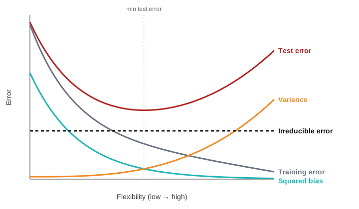
HW1 Q2 五条曲线与偏差-方差分解(a) 画出随灵活度增加时的 squared bias、variance、training error、test error、irreducible error 五条曲线;(b) 解释形状;(c) 证明 E [ f ( x 0 ) − f ^ ( x 0 ) ] 2 = Var ( f ^ ( x 0 ) ) + [ Bias ( f ^ ( x 0 ) ) ] 2 E[f(x_0)-\hat f(x_0)]^2=\operatorname{Var}(\hat f(x_0))+[\operatorname{Bias}(\hat f(x_0))]^2 E [ f ( x 0 ) − f ^ ( x 0 ) ] 2 = Var ( f ^ ( x 0 )) + [ Bias ( f ^ ( x 0 )) ] 2
查看答案
(a)(b)
Squared bias :单调下降。模型越灵活,越能逼近真实 f f f Variance :单调上升。越灵活,换一份训练集拟合结果变化越大。Training error :单调下降。灵活模型能越来越贴合训练点。Test error :U 形。先因 bias 下降而下降,后因 variance 上升而上升。Irreducible error :水平线 Var ( ε ) \operatorname{Var}(\varepsilon) Var ( ε )
五条曲线示意图:test error = squared bias + variance + irreducible error,在竖虚线处最小。
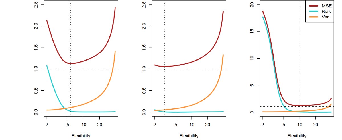
课件里的三个例子:红线 test MSE,蓝线 squared bias,橙线 variance,水平虚线 Var(ε)。(Lecture 02 p.45)
(c) 记 f ˉ = E [ f ^ ( x 0 ) ] \bar f=E[\hat f(x_0)] f ˉ = E [ f ^ ( x 0 )]
E [ f − f ^ ] 2 = E [ ( f − f ˉ ) + ( f ˉ − f ^ ) ] 2 = ( f − f ˉ ) 2 + 2 ( f − f ˉ ) E [ f ˉ − f ^ ] + E [ f ˉ − f ^ ] 2 E[f-\hat f]^2=E[(f-\bar f)+(\bar f-\hat f)]^2=(f-\bar f)^2+2(f-\bar f)\,E[\bar f-\hat f]+E[\bar f-\hat f]^2 E [ f − f ^ ] 2 = E [( f − f ˉ ) + ( f ˉ − f ^ ) ] 2 = ( f − f ˉ ) 2 + 2 ( f − f ˉ ) E [ f ˉ − f ^ ] + E [ f ˉ − f ^ ] 2 因为 f f f f ˉ \bar f f ˉ E [ f ˉ − f ^ ] = 0 E[\bar f-\hat f]=0 E [ f ˉ − f ^ ] = 0
E [ f − f ^ ] 2 = [ Bias ( f ^ ) ] 2 + Var ( f ^ ) E[f-\hat f]^2=[\operatorname{Bias}(\hat f)]^2+\operatorname{Var}(\hat f) E [ f − f ^ ] 2 = [ Bias ( f ^ ) ] 2 + Var ( f ^ )
课件对应:Lecture 02 p.42–45(The Bias-Variance Trade-Off),p.38–39(Overfitting 的两个例子)。
2. 线性回归的矩阵形式与系数推断
核心公式
y = X β + ε , β ^ = ( X ′ X ) − 1 X ′ y \mathbf y=X\boldsymbol\beta+\boldsymbol\varepsilon,\qquad \hat{\boldsymbol\beta}=(X'X)^{-1}X'\mathbf y y = X β + ε , β ^ = ( X ′ X ) − 1 X ′ y Cov ( β ^ ) = σ 2 ( X ′ X ) − 1 = σ 2 C , Var ( β ^ j ) = σ 2 C j j , s e ( β ^ j ) = σ ^ 2 C j j \operatorname{Cov}(\hat{\boldsymbol\beta})=\sigma^2(X'X)^{-1}=\sigma^2C,\qquad \operatorname{Var}(\hat\beta_j)=\sigma^2C_{jj},\qquad se(\hat\beta_j)=\sqrt{\hat\sigma^2C_{jj}} Cov ( β ^ ) = σ 2 ( X ′ X ) − 1 = σ 2 C , Var ( β ^ j ) = σ 2 C j j , se ( β ^ j ) = σ ^ 2 C j j
注意 X X X 第一列全是 1 (对应截距),所以 ( X ′ X ) − 1 (X'X)^{-1} ( X ′ X ) − 1 ( k + 1 ) × ( k + 1 ) (k+1)\times(k+1) ( k + 1 ) × ( k + 1 )
单个系数的 t 检验:t 0 = β ^ j / s e ( β ^ j ) t_0=\hat\beta_j/se(\hat\beta_j) t 0 = β ^ j / se ( β ^ j ) n − p n-p n − p p = k + 1 p=k+1 p = k + 1
Exam Q1 由 ( X ′ X ) − 1 (X'X)^{-1} ( X ′ X ) − 1 ( X ′ X ) − 1 = [ 0.893758 − 0.028245 − 0.0175641 − 0.028245 0.0013329 0.0001547 − 0.0175641 0.0001547 0.0009108 ] (X'X)^{-1}=\begin{bmatrix}0.893758&-0.028245&-0.0175641\\-0.028245&0.0013329&0.0001547\\-0.0175641&0.0001547&0.0009108\end{bmatrix} ( X ′ X ) − 1 = 0.893758 − 0.028245 − 0.0175641 − 0.028245 0.0013329 0.0001547 − 0.0175641 0.0001547 0.0009108 (a) 回归模型中有几个变量?(b) 如果 σ ^ 2 = 50 \hat\sigma^2=50 σ ^ 2 = 50
查看答案
(a) 矩阵是 3 × 3 3\times3 3 × 3 β 0 , β 1 , β 2 \beta_0,\beta_1,\beta_2 β 0 , β 1 , β 2 2 个预测变量 (外加截距)。
(b) Var ( β ^ j ) = σ ^ 2 C j j \operatorname{Var}(\hat\beta_j)=\hat\sigma^2C_{jj} Var ( β ^ j ) = σ ^ 2 C j j
Var ( β ^ 0 ) = 50 ( 0.893758 ) = 44.69 , Var ( β ^ 1 ) = 50 ( 0.0013329 ) = 0.0666 , Var ( β ^ 2 ) = 50 ( 0.0009108 ) = 0.0455 \operatorname{Var}(\hat\beta_0)=50(0.893758)=44.69,\quad \operatorname{Var}(\hat\beta_1)=50(0.0013329)=0.0666,\quad \operatorname{Var}(\hat\beta_2)=50(0.0009108)=0.0455 Var ( β ^ 0 ) = 50 ( 0.893758 ) = 44.69 , Var ( β ^ 1 ) = 50 ( 0.0013329 ) = 0.0666 , Var ( β ^ 2 ) = 50 ( 0.0009108 ) = 0.0455 (c) s e ( β ^ 0 ) = 44.69 = 6.685 se(\hat\beta_0)=\sqrt{44.69}=6.685 se ( β ^ 0 ) = 44.69 = 6.685
易错点:非对角线元素是 协方差 Cov ( β ^ i , β ^ j ) = σ 2 C i j \operatorname{Cov}(\hat\beta_i,\hat\beta_j)=\sigma^2C_{ij} Cov ( β ^ i , β ^ j ) = σ 2 C ij
Lecture 04 p.17–19, 31 Wire bond 拉力数据(矩阵法)n = 25 n=25 n = 25 x 1 x_1 x 1 x 2 x_2 x 2 y y y
展开原始数据(25 个观测)
Obs x 1 x_1 x 1 x 2 x_2 x 2 y y y 1 2 50 9.95 2 8 110 24.45 3 11 120 31.75 4 10 550 35.00 5 8 295 25.02 6 4 200 16.86 7 2 375 14.38 8 2 52 9.60 9 9 100 24.35 10 8 300 27.50 11 4 412 17.08 12 11 400 37.00 13 12 500 41.95 14 2 360 11.66 15 4 205 21.65 16 4 400 17.89 17 20 600 69.00 18 1 585 10.30 19 10 540 34.93 20 15 250 46.59 21 15 290 44.88 22 16 510 54.12 23 17 590 56.63 24 6 100 22.13 25 5 400 21.15
由数据得
X ′ X = [ 25 206 8294 206 2396 77177 8294 77177 3531848 ] , X ′ y = [ 725.82 8008.47 274811.31 ] X'X=\begin{bmatrix}25&206&8294\\206&2396&77177\\8294&77177&3531848\end{bmatrix},\quad X'\mathbf y=\begin{bmatrix}725.82\\8008.47\\274811.31\end{bmatrix} X ′ X = 25 206 8294 206 2396 77177 8294 77177 3531848 , X ′ y = 725.82 8008.47 274811.31 求回归方程;并在 σ ^ 2 = M S E = 5.2352 \hat\sigma^2=MS_E=5.2352 σ ^ 2 = M S E = 5.2352 C 22 = 0.0000015 C_{22}=0.0000015 C 22 = 0.0000015 H 0 : β 2 = 0 H_0:\beta_2=0 H 0 : β 2 = 0 α = 0.05 \alpha=0.05 α = 0.05
查看答案
β ^ = ( X ′ X ) − 1 X ′ y = [ 0.214653 − 0.007491 − 0.000340 − 0.007491 0.001671 − 0.000019 − 0.000340 − 0.000019 0.0000015 ] [ 725.82 8008.47 274811.31 ] = [ 2.26379 2.74427 0.01253 ] \hat{\boldsymbol\beta}=(X'X)^{-1}X'\mathbf y=\begin{bmatrix}0.214653&-0.007491&-0.000340\\-0.007491&0.001671&-0.000019\\-0.000340&-0.000019&0.0000015\end{bmatrix}\begin{bmatrix}725.82\\8008.47\\274811.31\end{bmatrix}=\begin{bmatrix}2.26379\\2.74427\\0.01253\end{bmatrix} β ^ = ( X ′ X ) − 1 X ′ y = 0.214653 − 0.007491 − 0.000340 − 0.007491 0.001671 − 0.000019 − 0.000340 − 0.000019 0.0000015 725.82 8008.47 274811.31 = 2.26379 2.74427 0.01253 y ^ = 2.26379 + 2.74427 x 1 + 0.01253 x 2 \hat y=2.26379+2.74427x_1+0.01253x_2 y ^ = 2.26379 + 2.74427 x 1 + 0.01253 x 2 t 0 = β ^ 2 σ ^ 2 C 22 = 0.01253 5.2352 × 0.0000015 = 4.477 > t 0.025 , 22 = 2.074 t_0=\frac{\hat\beta_2}{\sqrt{\hat\sigma^2C_{22}}}=\frac{0.01253}{\sqrt{5.2352\times0.0000015}}=4.477>t_{0.025,22}=2.074 t 0 = σ ^ 2 C 22 β ^ 2 = 5.2352 × 0.0000015 0.01253 = 4.477 > t 0.025 , 22 = 2.074 拒绝 H 0 H_0 H 0
HW2 Q2 (a)(b) 轴承磨损数据y y y x 1 x_1 x 1 x 2 x_2 x 2
Obs y y y x 1 x_1 x 1 x 2 x_2 x 2 1 293 1.6 851 2 230 15.5 816 3 172 22.0 1058 4 91 43.0 1201 5 113 33.0 1357 6 125 40.0 1115
(a) 拟合 y = β 0 + β 1 x 1 + β 2 x 2 + ε y=\beta_0+\beta_1x_1+\beta_2x_2+\varepsilon y = β 0 + β 1 x 1 + β 2 x 2 + ε σ 2 \sigma^2 σ 2 α = 0.05 \alpha=0.05 α = 0.05
查看答案
(a) y ^ = 383.80 − 3.638 x 1 − 0.1117 x 2 \hat y=383.80-3.638\,x_1-0.1117\,x_2 y ^ = 383.80 − 3.638 x 1 − 0.1117 x 2
(b) S S E = 457.86 SSE=457.86 S S E = 457.86 σ ^ 2 = M S E = S S E / ( n − p ) = 457.86 / 3 = 152.62 \hat\sigma^2=MSE=SSE/(n-p)=457.86/3=152.62 σ ^ 2 = M S E = S S E / ( n − p ) = 457.86/3 = 152.62
系数 估计 t 结论(t 0.025 , 3 = 3.182 t_{0.025,3}=3.182 t 0.025 , 3 = 3.182 β 0 \beta_0 β 0 383.80 10.60 显著 β 1 \beta_1 β 1 −3.638 −6.42 显著 β 2 \beta_2 β 2 −0.1117 −2.57 不显著
3. ANOVA、R²、F 检验与 Extra Sum of Squares
核心公式 (n n n k k k p = k + 1 p=k+1 p = k + 1
S S T = S S R + S S E , R 2 = S S R S S T , R a d j 2 = 1 − S S E / ( n − p ) S S T / ( n − 1 ) SST=SSR+SSE,\qquad R^2=\frac{SSR}{SST},\qquad R^2_{adj}=1-\frac{SSE/(n-p)}{SST/(n-1)} S S T = S S R + S S E , R 2 = S S T S S R , R a d j 2 = 1 − S S T / ( n − 1 ) S S E / ( n − p ) F 0 = S S R / k S S E / ( n − p ) = M S R M S E ∼ F k , n − p , 拒绝 H 0 : β 1 = ⋯ = β k = 0 若 F 0 > F α , k , n − p F_0=\frac{SSR/k}{SSE/(n-p)}=\frac{MSR}{MSE}\sim F_{k,\,n-p},\qquad \text{拒绝 }H_0:\beta_1=\dots=\beta_k=0\text{ 若 }F_0>F_{\alpha,k,n-p} F 0 = S S E / ( n − p ) S S R / k = M S E M S R ∼ F k , n − p , 拒绝 H 0 : β 1 = ⋯ = β k = 0 若 F 0 > F α , k , n − p Partial F(extra sum of squares) :在已有模型上增加 r r r
F 0 = [ S S R ( full ) − S S R ( reduced ) ] / r M S E ( full ) ∼ F r , n − p f u l l F_0=\frac{\big[SSR(\text{full})-SSR(\text{reduced})\big]/r}{MSE(\text{full})}\sim F_{r,\,n-p_{full}} F 0 = M S E ( full ) [ S S R ( full ) − S S R ( reduced ) ] / r ∼ F r , n − p f u l l 分母一定用 完整模型(full model) 的 MSE。
Exam Q2 由平方和做整体检验和偏 F 检验模型有 2 个回归变量,20 个观测,S S T = 1000 SST=1000 S S T = 1000 S S R = 750 SSR=750 S S R = 750 R 2 R^2 R 2 R 2 R^2 R 2 α = 0.05 \alpha=0.05 α = 0.05 α = 0.01 \alpha=0.01 α = 0.01 S S R = 785 SSR=785 S S R = 785
查看答案
n = 20 n=20 n = 20 k = 2 k=2 k = 2 p = 3 p=3 p = 3 S S E = S S T − S S R = 250 SSE=SST-SSR=250 S S E = S S T − S S R = 250
(a) R 2 = 750 / 1000 = 0.75 R^2=750/1000=0.75 R 2 = 750/1000 = 0.75
(b) R a d j 2 = 1 − 250 / 17 1000 / 19 = 1 − 14.71 52.63 = 0.721 R^2_{adj}=1-\dfrac{250/17}{1000/19}=1-\dfrac{14.71}{52.63}=0.721 R a d j 2 = 1 − 1000/19 250/17 = 1 − 52.63 14.71 = 0.721
(c)
F 0 = 750 / 2 250 / 17 = 375 14.71 = 25.5 F_0=\frac{750/2}{250/17}=\frac{375}{14.71}=25.5 F 0 = 250/17 750/2 = 14.71 375 = 25.5 F 0.05 , 2 , 17 = 3.59 F_{0.05,2,17}=3.59 F 0.05 , 2 , 17 = 3.59 F 0.01 , 2 , 17 = 6.11 F_{0.01,2,17}=6.11 F 0.01 , 2 , 17 = 6.11 α \alpha α F 0 > F F_0>F F 0 > F 拒绝 H 0 : β 1 = β 2 = 0 H_0:\beta_1=\beta_2=0 H 0 : β 1 = β 2 = 0
(d) 新模型 k = 3 k=3 k = 3 p = 4 p=4 p = 4 S S R f u l l = 785 SSR_{full}=785 S S R f u l l = 785 S S E f u l l = 1000 − 785 = 215 SSE_{full}=1000-785=215 S S E f u l l = 1000 − 785 = 215 M S E f u l l = 215 / 16 = 13.44 MSE_{full}=215/16=13.44 M S E f u l l = 215/16 = 13.44
F 0 = ( 785 − 750 ) / 1 215 / 16 = 35 13.44 = 2.60 < F 0.05 , 1 , 16 = 4.49 F_0=\frac{(785-750)/1}{215/16}=\frac{35}{13.44}=2.60<F_{0.05,1,16}=4.49 F 0 = 215/16 ( 785 − 750 ) /1 = 13.44 35 = 2.60 < F 0.05 , 1 , 16 = 4.49 不能拒绝 H 0 : β 3 = 0 H_0:\beta_3=0 H 0 : β 3 = 0 R 2 R^2 R 2 R 2 R^2 R 2
Lecture 04 p.26–27 Wire bond 的 ANOVA 表
查看答案
来源 SS df MS f 0 f_0 f 0 Regression 5990.7712 2 2995.3856 572.17 Error 115.1735 22 5.2352 Total 6105.9447 24
f 0 = 572.17 > f 0.05 , 2 , 22 = 3.44 f_0=572.17>f_{0.05,2,22}=3.44 f 0 = 572.17 > f 0.05 , 2 , 22 = 3.44 1.08 × 10 − 19 1.08\times10^{-19} 1.08 × 1 0 − 19 H 0 H_0 H 0
Lecture 04 p.69–71 加入 x 3 , x 4 x_3,x_4 x 3 , x 4 Wire bond 数据,已有 x 1 , x 2 x_1,x_2 x 1 , x 2 S S R ( β 2 , β 1 ∣ β 0 ) = 5990.8 SSR(\beta_2,\beta_1|\beta_0)=5990.8 S S R ( β 2 , β 1 ∣ β 0 ) = 5990.8 x 3 , x 4 x_3,x_4 x 3 , x 4 S S R ( β 4 , β 3 , β 2 , β 1 ∣ β 0 ) = 6024.0 SSR(\beta_4,\beta_3,\beta_2,\beta_1|\beta_0)=6024.0 S S R ( β 4 , β 3 , β 2 , β 1 ∣ β 0 ) = 6024.0 M S E = 4.1 MSE=4.1 M S E = 4.1 n = 25 n=25 n = 25 x 3 , x 4 x_3,x_4 x 3 , x 4
查看答案
S S R ( β 4 , β 3 ∣ β 2 , β 1 , β 0 ) = 6024.0 − 5990.8 = 33.2 ( 2 个自由度 ) SSR(\beta_4,\beta_3|\beta_2,\beta_1,\beta_0)=6024.0-5990.8=33.2\quad(2\text{ 个自由度}) S S R ( β 4 , β 3 ∣ β 2 , β 1 , β 0 ) = 6024.0 − 5990.8 = 33.2 ( 2 个自由度 ) f 0 = 33.2 / 2 4.1 = 4.05 > f 0.05 , 2 , 20 = 3.49 f_0=\frac{33.2/2}{4.1}=4.05>f_{0.05,2,20}=3.49 f 0 = 4.1 33.2/2 = 4.05 > f 0.05 , 2 , 20 = 3.49 拒绝 H 0 H_0 H 0 x 3 , x 4 x_3,x_4 x 3 , x 4 至少一个 有显著贡献。分母自由度 n − p = 25 − 5 = 20 n-p=25-5=20 n − p = 25 − 5 = 20
HW2 Q1 补全回归输出表考虑下面的计算机输出:
The regression equation is Y = 254 + 2.77 x1 − 3.58 x2
Predictor Coef SE Coef T Constant 253.810 4.781 ? x1 2.7738 0.1846 15.02 x2 −3.5753 0.1526 ?
S = 5.05756 R-Sq = ? R-Sq (adj) = 98.4%
Analysis of Variance
Source DF SS MS F Regression 2 22784 11392 ? Residual error ? ? ? Total 14 23091
(a) 补全缺失值;(b) 回归显著性的结论;(c) 各回归变量的贡献。
查看答案
(a) n = 15 n=15 n = 15
T c o n s t = 253.810 / 4.781 = 53.09 T_{const}=253.810/4.781=53.09 T co n s t = 253.810/4.781 = 53.09 T x 2 = − 3.5753 / 0.1526 = − 23.43 T_{x_2}=-3.5753/0.1526=-23.43 T x 2 = − 3.5753/0.1526 = − 23.43 Residual DF = 14 − 2 = 12 =14-2=12 = 14 − 2 = 12 S S E = 23091 − 22784 = 307 SSE=23091-22784=307 S S E = 23091 − 22784 = 307 M S E = 307 / 12 = 25.58 MSE=307/12=25.58 M S E = 307/12 = 25.58 S 2 = 5.05756 2 = 25.58 S^2=5.05756^2=25.58 S 2 = 5.0575 6 2 = 25.58
F = 11392 / 25.58 = 445.3 F=11392/25.58=445.3 F = 11392/25.58 = 445.3 R 2 = 22784 / 23091 = 98.7 % R^2=22784/23091=98.7\% R 2 = 22784/23091 = 98.7%
补全后的输出表:
Predictor Coef SE Coef T Constant 253.810 4.781 53.09 x1 2.7738 0.1846 15.02 x2 −3.5753 0.1526 −23.43
Source DF SS MS F Regression 2 22784 11392 445.3 Residual error 12 307 25.58 Total 14 23091
R-Sq = 98.7%
(b) F = 445.3 ≫ F 0.05 , 2 , 12 = 3.89 F=445.3\gg F_{0.05,2,12}=3.89 F = 445.3 ≫ F 0.05 , 2 , 12 = 3.89
(c) ∣ t ∣ |t| ∣ t ∣ t 0.025 , 12 = 2.179 t_{0.025,12}=2.179 t 0.025 , 12 = 2.179 x 1 x_1 x 1 x 2 x_2 x 2
HW2 Q2 (c)(e)(g) 轴承数据的整体检验与偏 F 检验
查看答案
(c) S S T = 30245.3 SST=30245.3 S S T = 30245.3 S S R = 29787.5 SSR=29787.5 S S R = 29787.5 F 0 = 29787.5 / 2 152.62 = 97.59 > F 0.05 , 2 , 3 = 9.55 F_0=\dfrac{29787.5/2}{152.62}=97.59>F_{0.05,2,3}=9.55 F 0 = 152.62 29787.5/2 = 97.59 > F 0.05 , 2 , 3 = 9.55
(d) x 1 = 25 , x 2 = 1000 x_1=25,\ x_2=1000 x 1 = 25 , x 2 = 1000 y ^ = 383.80 − 3.638 ( 25 ) − 0.1117 ( 1000 ) = 181.2 \hat y=383.80-3.638(25)-0.1117(1000)=181.2 y ^ = 383.80 − 3.638 ( 25 ) − 0.1117 ( 1000 ) = 181.2
(e) 只有 x 1 x_1 x 1 S S E = 1469.5 SSE=1469.5 S S E = 1469.5
F 0 = 1469.5 − 457.9 152.62 = 6.63 < F 0.05 , 1 , 3 = 10.13 ( P = 0.082 ) F_0=\frac{1469.5-457.9}{152.62}=6.63<F_{0.05,1,3}=10.13\ (P=0.082) F 0 = 152.62 1469.5 − 457.9 = 6.63 < F 0.05 , 1 , 3 = 10.13 ( P = 0.082 ) 在已有 x 1 x_1 x 1 不显著 。
(f) 加交互项 x 1 x 2 x_1x_2 x 1 x 2 y ^ = 483.97 − 7.656 x 1 − 0.2221 x 2 + 0.004087 x 1 x 2 \hat y=483.97-7.656x_1-0.2221x_2+0.004087x_1x_2 y ^ = 483.97 − 7.656 x 1 − 0.2221 x 2 + 0.004087 x 1 x 2 S S E = 293.98 SSE=293.98 S S E = 293.98 F 0 = 67.92 > F 0.05 , 3 , 2 = 19.16 F_0=67.92>F_{0.05,3,2}=19.16 F 0 = 67.92 > F 0.05 , 3 , 2 = 19.16
(g) F 0 = 457.86 − 293.98 293.98 / 2 = 1.11 < F 0.05 , 1 , 2 = 18.51 F_0=\dfrac{457.86-293.98}{293.98/2}=1.11<F_{0.05,1,2}=18.51 F 0 = 293.98/2 457.86 − 293.98 = 1.11 < F 0.05 , 1 , 2 = 18.51 不显著 。
HW2 Q3 由 R 2 R^2 R 2 C p C_p C p 30 个观测,完整模型 9 个回归变量,σ ^ 2 = M S E = 100 \hat\sigma^2=MSE=100 σ ^ 2 = M S E = 100 R 2 = 0.92 R^2=0.92 R 2 = 0.92 α = 0.05 \alpha=0.05 α = 0.05 S S E = 2200 SSE=2200 S S E = 2200 σ 2 \sigma^2 σ 2 C p C_p C p
查看答案
(a) S S E = M S E ( n − p ) = 100 × 20 = 2000 SSE=MSE(n-p)=100\times20=2000 S S E = M S E ( n − p ) = 100 × 20 = 2000 S S T = S S E / ( 1 − R 2 ) = 2000 / 0.08 = 25000 SST=SSE/(1-R^2)=2000/0.08=25000 S S T = S S E / ( 1 − R 2 ) = 2000/0.08 = 25000 S S R = 23000 SSR=23000 S S R = 23000
F 0 = 23000 / 9 100 = 25.56 > F 0.05 , 9 , 20 = 2.39 F_0=\frac{23000/9}{100}=25.56>F_{0.05,9,20}=2.39 F 0 = 100 23000/9 = 25.56 > F 0.05 , 9 , 20 = 2.39 拒绝 H 0 H_0 H 0
(b) σ ^ r e d u c e d 2 = 2200 / ( 30 − 5 ) = 88 < 100 \hat\sigma^2_{reduced}=2200/(30-5)=88<100 σ ^ r e d u ce d 2 = 2200/ ( 30 − 5 ) = 88 < 100 更好 。
(c) C p = S S E p σ ^ f u l l 2 − n + 2 p = 2200 100 − 30 + 2 ( 5 ) = 2 C_p=\dfrac{SSE_p}{\hat\sigma^2_{full}}-n+2p=\dfrac{2200}{100}-30+2(5)=2 C p = σ ^ f u l l 2 S S E p − n + 2 p = 100 2200 − 30 + 2 ( 5 ) = 2 C p = 2 ≤ p = 5 C_p=2\le p=5 C p = 2 ≤ p = 5
4. Logistic 回归
核心公式
p ( X ) = Pr ( Y = 1 ∣ X ) = e β 0 + β 1 X 1 + ⋯ + β p X p 1 + e β 0 + β 1 X 1 + ⋯ + β p X p , log p ( X ) 1 − p ( X ) = β 0 + β 1 X 1 + ⋯ + β p X p p(X)=\Pr(Y=1\mid X)=\frac{e^{\beta_0+\beta_1X_1+\cdots+\beta_pX_p}}{1+e^{\beta_0+\beta_1X_1+\cdots+\beta_pX_p}},\qquad \log\frac{p(X)}{1-p(X)}=\beta_0+\beta_1X_1+\cdots+\beta_pX_p p ( X ) = Pr ( Y = 1 ∣ X ) = 1 + e β 0 + β 1 X 1 + ⋯ + β p X p e β 0 + β 1 X 1 + ⋯ + β p X p , log 1 − p ( X ) p ( X ) = β 0 + β 1 X 1 + ⋯ + β p X p
β j \beta_j β j X j X_j X j log-odds 增加 β j \beta_j β j e β j e^{\beta_j} e β j p ( X ) = 0.5 p(X)=0.5 p ( X ) = 0.5 = 0 =0 = 0 Bernoulli PMF:P ( y ) = p y ( 1 − p ) 1 − y P(y)=p^y(1-p)^{1-y} P ( y ) = p y ( 1 − p ) 1 − y y ∈ { 0 , 1 } y\in\{0,1\} y ∈ { 0 , 1 }
Exam Q5 学习时长、GPA 与拿 A 的概率X 1 X_1 X 1 X 2 X_2 X 2 Y Y Y β ^ 0 = − 6 \hat\beta_0=-6 β ^ 0 = − 6 β ^ 1 = 0.05 \hat\beta_1=0.05 β ^ 1 = 0.05 β ^ 2 = 1 \hat\beta_2=1 β ^ 2 = 1
查看答案
(a) η = − 6 + 0.05 ( 40 ) + 1 ( 3.5 ) = − 0.5 \eta=-6+0.05(40)+1(3.5)=-0.5 η = − 6 + 0.05 ( 40 ) + 1 ( 3.5 ) = − 0.5
p ^ = e − 0.5 1 + e − 0.5 = 0.3775 \hat p=\frac{e^{-0.5}}{1+e^{-0.5}}=0.3775 p ^ = 1 + e − 0.5 e − 0.5 = 0.3775 (b) p = 0.5 ⟺ η = 0 p=0.5\iff\eta=0 p = 0.5 ⟺ η = 0 − 6 + 0.05 h + 3.5 = 0 ⇒ h = 50 -6+0.05h+3.5=0\Rightarrow h=50 − 6 + 0.05 h + 3.5 = 0 ⇒ h = 50
Exam Q7 类别编码为 { − 1 , 1 } \{-1,1\} { − 1 , 1 } 类别编码为 ( 0 , 1 ) (0,1) ( 0 , 1 ) Pr ( y = 1 ∣ X ) = e X β 1 + e X β \Pr(y=1|X)=\dfrac{e^{X\beta}}{1+e^{X\beta}} Pr ( y = 1∣ X ) = 1 + e X β e X β Pr ( y = 0 ∣ X ) = 1 1 + e X β \Pr(y=0|X)=\dfrac{1}{1+e^{X\beta}} Pr ( y = 0∣ X ) = 1 + e X β 1 ( − 1 , 1 ) (-1,1) ( − 1 , 1 ) Pr ( y = 1 or − 1 ∣ X ) = 1 1 + e − y ( X β ) \Pr(y=1\text{ or }-1\mid X)=\dfrac{1}{1+e^{-y(X\beta)}} Pr ( y = 1 or − 1 ∣ X ) = 1 + e − y ( X β ) 1 y ∈ { − 1 , 1 } y\in\{-1,1\} y ∈ { − 1 , 1 }
查看答案
分子分母同除 e X β e^{X\beta} e X β
Pr ( y = 1 ∣ X ) = e X β 1 + e X β = 1 1 + e − X β , Pr ( y = − 1 ∣ X ) = 1 1 + e X β = 1 1 + e − ( − 1 ) X β \Pr(y=1|X)=\frac{e^{X\beta}}{1+e^{X\beta}}=\frac{1}{1+e^{-X\beta}},\qquad \Pr(y=-1|X)=\frac{1}{1+e^{X\beta}}=\frac{1}{1+e^{-(-1)X\beta}} Pr ( y = 1∣ X ) = 1 + e X β e X β = 1 + e − X β 1 , Pr ( y = − 1∣ X ) = 1 + e X β 1 = 1 + e − ( − 1 ) X β 1 两式只差 X β X\beta X β y y y 1 1 + e − y X β \dfrac{1}{1+e^{-yX\beta}} 1 + e − y X β 1
Bernoulli PMF:y ∈ { 0 , 1 } y\in\{0,1\} y ∈ { 0 , 1 } P ( y ) = p y ( 1 − p ) 1 − y P(y)=p^y(1-p)^{1-y} P ( y ) = p y ( 1 − p ) 1 − y y ∈ { − 1 , 1 } y\in\{-1,1\} y ∈ { − 1 , 1 } 1 + y 2 ∈ { 0 , 1 } \frac{1+y}{2}\in\{0,1\} 2 1 + y ∈ { 0 , 1 }
P ( y ) = p 1 + y 2 ( 1 − p ) 1 − y 2 P(y)=p^{\frac{1+y}{2}}(1-p)^{\frac{1-y}{2}} P ( y ) = p 2 1 + y ( 1 − p ) 2 1 − y y = 1 y=1 y = 1 p p p y = − 1 y=-1 y = − 1 1 − p 1-p 1 − p
Lecture 05 p.11–12 Default 数据模型 1:Default ~ balance(p.11)
Coefficient Std. error z-statistic p-value Intercept −10.6513 0.3612 −29.5 <0.0001 balance 0.0055 0.0002 24.9 <0.0001
模型 2:Default ~ balance + income(千美元)+ student(p.12)
Coefficient Std. error z-statistic p-value Intercept −10.8690 0.4923 −22.08 <0.0001 balance 0.0057 0.0002 24.74 <0.0001 income 0.0030 0.0082 0.37 0.7115 student[Yes] −0.6468 0.2362 −2.74 0.0062
对照:只用 student(p.13,confounding)
Coefficient Std. error z-statistic p-value Intercept −3.5041 0.0707 −49.55 <0.0001 student[Yes] 0.4049 0.1150 3.52 0.0004
(1) 用模型 1,balance 为 1000 时违约概率?
(2) 用模型 2(课件计算时 balance 系数取 0.00574),balance 1500、income 40 的学生与非学生违约概率?
查看答案
(1) p ^ = e − 10.6513 + 0.0055 ( 1000 ) 1 + e − 10.6513 + 0.0055 ( 1000 ) = 0.00576 \hat p=\dfrac{e^{-10.6513+0.0055(1000)}}{1+e^{-10.6513+0.0055(1000)}}=0.00576 p ^ = 1 + e − 10.6513 + 0.0055 ( 1000 ) e − 10.6513 + 0.0055 ( 1000 ) = 0.00576
(2) 学生:η = − 10.869 + 0.00574 ( 1500 ) + 0.003 ( 40 ) − 0.6468 = − 2.786 \eta=-10.869+0.00574(1500)+0.003(40)-0.6468=-2.786 η = − 10.869 + 0.00574 ( 1500 ) + 0.003 ( 40 ) − 0.6468 = − 2.786 p ^ = 0.058 \hat p=0.058 p ^ = 0.058 η = − 2.139 \eta=-2.139 η = − 2.139 p ^ = 0.105 \hat p=0.105 p ^ = 0.105
同样的 balance 和 income 下,学生违约概率更低(student 系数为负)。课件 p.13 讲的 confounding:单独用 student 时系数为正,因为学生平均 balance 更高。
HW3 Q2 Titanic:Bernoulli 与 Binomial 两种响应格式(a) 用 Pclass、Sex、Age 拟合 logistic 回归(Bernoulli 格式);(b) 把 Age 按 5 岁分箱为 Age_Range 再拟合;(c) 按 Pclass、Sex、Age_Range 分组,转为 Binomial 格式(Survived、Died 两列)拟合;(d) 模型是否充分?
查看答案
(b) 与 (a) 不同 :Age 从连续变量变成分箱变量,模型的设计矩阵变了。
(c) 与 (b) 的 系数相同 :分组后每一行只是把相同预测变量组合下的 Bernoulli 观测合并成 Binomial 计数,似然函数相同(只差一个与参数无关的组合数常数),所以 MLE 一样;但 deviance 和自由度不同。
(d) 看 residual deviance 与自由度:Binomial 格式下 deviance/df 接近 1、拟合优度检验 P 值大,说明模型充分。
5. Bayes 分类器、LDA、QDA 与 KNN
核心公式
Pr ( Y = k ∣ X = x ) = π k f k ( x ) ∑ l = 1 K π l f l ( x ) , f k ( x ) = 1 2 π σ k exp ( − ( x − μ k ) 2 2 σ k 2 ) \Pr(Y=k\mid X=x)=\frac{\pi_kf_k(x)}{\sum_{l=1}^K\pi_lf_l(x)},\qquad f_k(x)=\frac{1}{\sqrt{2\pi}\sigma_k}\exp\Big(-\frac{(x-\mu_k)^2}{2\sigma_k^2}\Big) Pr ( Y = k ∣ X = x ) = ∑ l = 1 K π l f l ( x ) π k f k ( x ) , f k ( x ) = 2 π σ k 1 exp ( − 2 σ k 2 ( x − μ k ) 2 )
LDA :各类方差相同 σ 1 2 = ⋯ = σ K 2 = σ 2 \sigma_1^2=\dots=\sigma_K^2=\sigma^2 σ 1 2 = ⋯ = σ K 2 = σ 2 δ k ( x ) = x μ k σ 2 − μ k 2 2 σ 2 + log π k \delta_k(x)=x\dfrac{\mu_k}{\sigma^2}-\dfrac{\mu_k^2}{2\sigma^2}+\log\pi_k δ k ( x ) = x σ 2 μ k − 2 σ 2 μ k 2 + log π k x x x QDA :各类方差不同,判别函数含 x 2 x^2 x 2 LDA bias 高、variance 低;QDA bias 低、variance 高。数据少时偏向 LDA,数据多或边界非线性时偏向 QDA。
KNN :K K K K K K
Exam Q3 LDA 还是 QDA?(a) 如果 Bayes 决策边界是线性的,LDA 和 QDA 哪个在训练集上表现更好?测试集呢?
(b) 如果边界是非线性的呢?
(c) 一般来说,随着样本量 n n n
查看答案
(a) 训练集:QDA 更好(更灵活,能拟合噪声)。测试集:LDA 更好(QDA 多出来的参数只带来过拟合)。
(b) 训练集和测试集都是 QDA 更好。
(c) 提高 。n n n
(d) 错 。边界是线性时,QDA 的额外灵活性不会降低 bias,只会增加 variance(样本少时尤其明显),测试错误率通常比 LDA 更高。
Exam Q6 用 Bayes 公式预测是否分红用去年利润百分比 X X X X ˉ = 10 \bar X=10 X ˉ = 10 X ˉ = 0 \bar X=0 X ˉ = 0 σ ^ 2 = 36 \hat\sigma^2=36 σ ^ 2 = 36 X X X X = 4 X=4 X = 4
查看答案
π y e s = 0.8 \pi_{yes}=0.8 π y es = 0.8 π n o = 0.2 \pi_{no}=0.2 π n o = 0.2 μ y e s = 10 \mu_{yes}=10 μ y es = 10 μ n o = 0 \mu_{no}=0 μ n o = 0 σ 2 = 36 \sigma^2=36 σ 2 = 36 1 2 π σ \frac{1}{\sqrt{2\pi}\sigma} 2 π σ 1
Pr ( yes ∣ X = 4 ) = 0.8 e − ( 4 − 10 ) 2 / 72 0.8 e − ( 4 − 10 ) 2 / 72 + 0.2 e − ( 4 − 0 ) 2 / 72 = 0.8 ( 0.6065 ) 0.8 ( 0.6065 ) + 0.2 ( 0.8007 ) = 0.4852 0.6453 = 0.752 \Pr(\text{yes}\mid X=4)=\frac{0.8\,e^{-(4-10)^2/72}}{0.8\,e^{-(4-10)^2/72}+0.2\,e^{-(4-0)^2/72}}=\frac{0.8(0.6065)}{0.8(0.6065)+0.2(0.8007)}=\frac{0.4852}{0.6453}=0.752 Pr ( yes ∣ X = 4 ) = 0.8 e − ( 4 − 10 ) 2 /72 + 0.2 e − ( 4 − 0 ) 2 /72 0.8 e − ( 4 − 10 ) 2 /72 = 0.8 ( 0.6065 ) + 0.2 ( 0.8007 ) 0.8 ( 0.6065 ) = 0.6453 0.4852 = 0.752
HW3 Q1 证明 QDA(p = 1)的 Bayes 分类器是二次的X ∣ Y = k ∼ N ( μ k , σ k 2 ) X\mid Y=k\sim N(\mu_k,\sigma_k^2) X ∣ Y = k ∼ N ( μ k , σ k 2 ) x x x
查看答案
Bayes 分类器选使 π k f k ( x ) \pi_kf_k(x) π k f k ( x ) k k k
log ( π k f k ( x ) ) = log π k − log σ k − 1 2 log ( 2 π ) − ( x − μ k ) 2 2 σ k 2 \log\big(\pi_kf_k(x)\big)=\log\pi_k-\log\sigma_k-\tfrac12\log(2\pi)-\frac{(x-\mu_k)^2}{2\sigma_k^2} log ( π k f k ( x ) ) = log π k − log σ k − 2 1 log ( 2 π ) − 2 σ k 2 ( x − μ k ) 2 去掉与 k k k − 1 2 log ( 2 π ) -\frac12\log(2\pi) − 2 1 log ( 2 π )
δ k ( x ) = − x 2 2 σ k 2 + μ k x σ k 2 − μ k 2 2 σ k 2 − log σ k + log π k \delta_k(x)=-\frac{x^2}{2\sigma_k^2}+\frac{\mu_kx}{\sigma_k^2}-\frac{\mu_k^2}{2\sigma_k^2}-\log\sigma_k+\log\pi_k δ k ( x ) = − 2 σ k 2 x 2 + σ k 2 μ k x − 2 σ k 2 μ k 2 − log σ k + log π k 因为 σ k \sigma_k σ k x 2 x^2 x 2 − 1 2 σ k 2 -\frac{1}{2\sigma_k^2} − 2 σ k 2 1 δ k ( x ) \delta_k(x) δ k ( x ) δ k ( x ) = δ l ( x ) \delta_k(x)=\delta_l(x) δ k ( x ) = δ l ( x ) x x x 二次 函数。若 σ k = σ \sigma_k=\sigma σ k = σ x 2 x^2 x 2
Lecture 06 p.11 LDA 一维例子
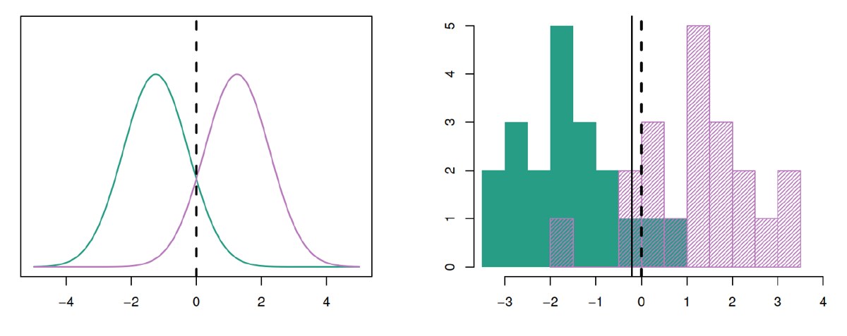
左:两类真实密度,虚线是 Bayes 边界 x = 0。右:每类 20 个样本的直方图,实线是 LDA 估计的边界。(Lecture 06 p.11)
μ 1 = − 1.5 \mu_1=-1.5 μ 1 = − 1.5 μ 2 = 1.5 \mu_2=1.5 μ 2 = 1.5 π 1 = π 2 = 0.5 \pi_1=\pi_2=0.5 π 1 = π 2 = 0.5 σ 2 = 1 \sigma^2=1 σ 2 = 1
查看答案
令 δ 1 ( x ) = δ 2 ( x ) \delta_1(x)=\delta_2(x) δ 1 ( x ) = δ 2 ( x ) π \pi π x = μ 1 + μ 2 2 = 0 x=\dfrac{\mu_1+\mu_2}{2}=0 x = 2 μ 1 + μ 2 = 0 x < 0 x<0 x < 0
HW1 Q5 KNN 手算6 个训练观测:
Obs X 1 X_1 X 1 X 2 X_2 X 2 X 3 X_3 X 3 Y 1 0 3 0 Red 2 2 0 0 Red 3 0 1 3 Red 4 0 1 2 Green 5 −1 0 1 Green 6 1 1 1 Red
在 X 1 = X 2 = X 3 = 0 X_1=X_2=X_3=0 X 1 = X 2 = X 3 = 0 K = 1 K=1 K = 1 K = 3 K=3 K = 3 K K K
查看答案
(a) 距离:Obs1 = 3,Obs2 = 2,Obs3 = 10 \sqrt{10} 10 5 \sqrt5 5 2 \sqrt2 2 3 \sqrt3 3
(b) K = 1 K=1 K = 1 Green 。K = 3 K=3 K = 3 Red (2/3)。
(c) 取 小 的 K K K K K K K K K
This page opens with a formula sheet covering all 6 lectures, then groups the 7 exam practice questions into 5 topics. Each topic starts with the key formulas, then the exam question, then the matching lecture examples and homework problems. Click Show answer to unfold a solution.
0. Formula sheet (Lectures 01–06)
In lecture order, with slide page numbers in brackets. Read it top to bottom before the exam.
Lecture 01 · Probability and statistics review
Common distributions
Distribution PMF / PDF E ( X ) E(X) E ( X ) Var ( X ) \operatorname{Var}(X) Var ( X ) Bernoulli( p ) (p) ( p ) p ( x ) = p x ( 1 − p ) 1 − x , x ∈ { 0 , 1 } p(x)=p^x(1-p)^{1-x},\ x\in\{0,1\} p ( x ) = p x ( 1 − p ) 1 − x , x ∈ { 0 , 1 } p p p p ( 1 − p ) p(1-p) p ( 1 − p ) Binomial( n , p ) (n,p) ( n , p ) ( n x ) p x ( 1 − p ) n − x \binom{n}{x}p^x(1-p)^{n-x} ( x n ) p x ( 1 − p ) n − x n p np n p n p ( 1 − p ) np(1-p) n p ( 1 − p ) Poisson( λ ) (\lambda) ( λ ) e − λ λ x x ! \dfrac{e^{-\lambda}\lambda^x}{x!} x ! e − λ λ x λ \lambda λ λ \lambda λ Normal( μ , σ 2 ) (\mu,\sigma^2) ( μ , σ 2 ) 1 σ 2 π exp [ − ( x − μ ) 2 2 σ 2 ] \dfrac{1}{\sigma\sqrt{2\pi}}\exp\!\Big[-\dfrac{(x-\mu)^2}{2\sigma^2}\Big] σ 2 π 1 exp [ − 2 σ 2 ( x − μ ) 2 ] μ \mu μ σ 2 \sigma^2 σ 2
Poisson process (p.59): P ( N ( t ) = n ) = ( λ t ) n e − λ t n ! P(N(t)=n)=\dfrac{(\lambda t)^ne^{-\lambda t}}{n!} P ( N ( t ) = n ) = n ! ( λ t ) n e − λ t E [ N ( t ) ] = λ t E[N(t)]=\lambda t E [ N ( t )] = λ t
Standardizing (p.66, 86): Z = X − μ σ ∼ N ( 0 , 1 ) Z=\dfrac{X-\mu}{\sigma}\sim N(0,1) Z = σ X − μ ∼ N ( 0 , 1 ) Φ ( t ) = P ( Z < t ) \Phi(t)=P(Z<t) Φ ( t ) = P ( Z < t )
Conditional probability and Bayes’ formula (pp.70–71)
P ( A ∣ B ) = P ( A B ) P ( B ) , P ( B ∣ A ) = P ( A ∣ B ) P ( B ) P ( A ) , P ( A ) = ∑ i P ( A ∣ B i ) P ( B i ) P(A\mid B)=\frac{P(AB)}{P(B)},\qquad P(B\mid A)=\frac{P(A\mid B)P(B)}{P(A)},\qquad P(A)=\sum_iP(A\mid B_i)P(B_i) P ( A ∣ B ) = P ( B ) P ( A B ) , P ( B ∣ A ) = P ( A ) P ( A ∣ B ) P ( B ) , P ( A ) = i ∑ P ( A ∣ B i ) P ( B i ) Expectation and variance (pp.76–84)
E ( X ) = ∑ x x p ( x ) or ∫ − ∞ ∞ x f ( x ) d x , Var ( X ) = E [ ( X − μ ) 2 ] = E ( X 2 ) − [ E ( X ) ] 2 E(X)=\sum_x x\,p(x)\ \ \text{or}\ \ \int_{-\infty}^{\infty}x f(x)\,dx,\qquad \operatorname{Var}(X)=E[(X-\mu)^2]=E(X^2)-[E(X)]^2 E ( X ) = x ∑ x p ( x ) or ∫ − ∞ ∞ x f ( x ) d x , Var ( X ) = E [( X − μ ) 2 ] = E ( X 2 ) − [ E ( X ) ] 2 E ( a X + b ) = a E ( X ) + b , Var ( a X + b ) = a 2 Var ( X ) , σ a X + b = ∣ a ∣ σ X E(aX+b)=aE(X)+b,\qquad \operatorname{Var}(aX+b)=a^2\operatorname{Var}(X),\qquad \sigma_{aX+b}=|a|\sigma_X E ( a X + b ) = a E ( X ) + b , Var ( a X + b ) = a 2 Var ( X ) , σ a X + b = ∣ a ∣ σ X Covariance and correlation (p.85)
Cov ( X , Y ) = E [ ( X − μ X ) ( Y − μ Y ) ] , ρ = σ X Y σ X σ Y ∈ [ − 1 , 1 ] \operatorname{Cov}(X,Y)=E[(X-\mu_X)(Y-\mu_Y)],\qquad \rho=\frac{\sigma_{XY}}{\sigma_X\sigma_Y}\in[-1,1] Cov ( X , Y ) = E [( X − μ X ) ( Y − μ Y )] , ρ = σ X σ Y σ X Y ∈ [ − 1 , 1 ] Var ( X ± Y ) = Var ( X ) + Var ( Y ) ± 2 Cov ( X , Y ) \operatorname{Var}(X\pm Y)=\operatorname{Var}(X)+\operatorname{Var}(Y)\pm2\operatorname{Cov}(X,Y) Var ( X ± Y ) = Var ( X ) + Var ( Y ) ± 2 Cov ( X , Y ) Independent ⇒ Cov = 0 \operatorname{Cov}=0 Cov = 0
Lecture 02 · Predictive modeling basics
Model and error decomposition (pp.17, 44)
Y = f ( X ) + ε , E [ ( Y − Y ^ ) 2 ] = [ f ( X ) − f ^ ( X ) ] 2 ⏟ reducible + Var ( ε ) ⏟ irreducible Y=f(X)+\varepsilon,\qquad E\big[(Y-\hat Y)^2\big]=\underbrace{[f(X)-\hat f(X)]^2}_{\text{reducible}}+\underbrace{\operatorname{Var}(\varepsilon)}_{\text{irreducible}} Y = f ( X ) + ε , E [ ( Y − Y ^ ) 2 ] = reducible [ f ( X ) − f ^ ( X ) ] 2 + irreducible Var ( ε ) MSE and the bias-variance decomposition (pp.34, 42–44)
M S E = 1 n ∑ i = 1 n ( y i − f ^ ( x i ) ) 2 , E [ ( y 0 − f ^ ( x 0 ) ) 2 ] = Var ( f ^ ( x 0 ) ) + [ Bias ( f ^ ( x 0 ) ) ] 2 + Var ( ε ) MSE=\frac1n\sum_{i=1}^n\big(y_i-\hat f(x_i)\big)^2,\qquad E\big[(y_0-\hat f(x_0))^2\big]=\operatorname{Var}(\hat f(x_0))+[\operatorname{Bias}(\hat f(x_0))]^2+\operatorname{Var}(\varepsilon) M S E = n 1 i = 1 ∑ n ( y i − f ^ ( x i ) ) 2 , E [ ( y 0 − f ^ ( x 0 ) ) 2 ] = Var ( f ^ ( x 0 )) + [ Bias ( f ^ ( x 0 )) ] 2 + Var ( ε ) Unbiased estimators (pp.40–41)
Definition: E ( Θ ^ ) = θ E(\hat\Theta)=\theta E ( Θ ^ ) = θ = E ( Θ ^ ) − θ =E(\hat\Theta)-\theta = E ( Θ ^ ) − θ
The sample mean is unbiased: X ˉ = 1 n ∑ X i \bar X=\dfrac1n\sum X_i X ˉ = n 1 ∑ X i E ( X ˉ ) = μ E(\bar X)=\mu E ( X ˉ ) = μ Var ( X ˉ ) = σ 2 n \operatorname{Var}(\bar X)=\dfrac{\sigma^2}{n} Var ( X ˉ ) = n σ 2
The sample variance is unbiased (divide by n − 1 n-1 n − 1 :
S 2 = 1 n − 1 ∑ i = 1 n ( X i − X ˉ ) 2 , E ( S 2 ) = σ 2 S^2=\frac{1}{n-1}\sum_{i=1}^n(X_i-\bar X)^2,\qquad E(S^2)=\sigma^2 S 2 = n − 1 1 i = 1 ∑ n ( X i − X ˉ ) 2 , E ( S 2 ) = σ 2 Proof sketch: E [ ∑ ( X i − X ˉ ) 2 ] = ∑ E ( X i 2 ) − n E ( X ˉ 2 ) = n ( σ 2 + μ 2 ) − n ( σ 2 n + μ 2 ) = ( n − 1 ) σ 2 E\big[\sum(X_i-\bar X)^2\big]=\sum E(X_i^2)-nE(\bar X^2)=n(\sigma^2+\mu^2)-n\big(\tfrac{\sigma^2}{n}+\mu^2\big)=(n-1)\sigma^2 E [ ∑ ( X i − X ˉ ) 2 ] = ∑ E ( X i 2 ) − n E ( X ˉ 2 ) = n ( σ 2 + μ 2 ) − n ( n σ 2 + μ 2 ) = ( n − 1 ) σ 2
The unbiased estimator with the smallest variance is the minimum variance unbiased estimator (MVUE) .
Classification error, Bayes classifier and KNN (pp.46–49)
Error rate = 1 n ∑ i = 1 n I ( y i ≠ y ^ i ) , Bayes: y ^ 0 = arg max j Pr ( Y = j ∣ X = x 0 ) \text{Error rate}=\frac1n\sum_{i=1}^nI(y_i\ne\hat y_i),\qquad \text{Bayes: }\hat y_0=\arg\max_j\Pr(Y=j\mid X=x_0) Error rate = n 1 i = 1 ∑ n I ( y i = y ^ i ) , Bayes: y ^ 0 = arg j max Pr ( Y = j ∣ X = x 0 ) Bayes error rate = 1 − E [ max j Pr ( Y = j ∣ X ) ] , KNN: Pr ( Y = j ∣ X = x 0 ) = 1 K ∑ i ∈ N 0 I ( y i = j ) \text{Bayes error rate}=1-E\Big[\max_j\Pr(Y=j\mid X)\Big],\qquad \text{KNN: }\Pr(Y=j\mid X=x_0)=\frac1K\sum_{i\in N_0}I(y_i=j) Bayes error rate = 1 − E [ j max Pr ( Y = j ∣ X ) ] , KNN: Pr ( Y = j ∣ X = x 0 ) = K 1 i ∈ N 0 ∑ I ( y i = j ) Lecture 03 · Simple linear regression
Model and least squares (pp.8–9)
Y = β 0 + β 1 x + ε , S x x = ∑ ( x i − x ˉ ) 2 = ∑ x i 2 − ( ∑ x i ) 2 n , S x y = ∑ ( x i − x ˉ ) ( y i − y ˉ ) = ∑ x i y i − ( ∑ x i ) ( ∑ y i ) n Y=\beta_0+\beta_1x+\varepsilon,\qquad S_{xx}=\sum(x_i-\bar x)^2=\sum x_i^2-\frac{(\sum x_i)^2}{n},\qquad S_{xy}=\sum(x_i-\bar x)(y_i-\bar y)=\sum x_iy_i-\frac{(\sum x_i)(\sum y_i)}{n} Y = β 0 + β 1 x + ε , S xx = ∑ ( x i − x ˉ ) 2 = ∑ x i 2 − n ( ∑ x i ) 2 , S x y = ∑ ( x i − x ˉ ) ( y i − y ˉ ) = ∑ x i y i − n ( ∑ x i ) ( ∑ y i ) β ^ 1 = S x y S x x , β ^ 0 = y ˉ − β ^ 1 x ˉ , e i = y i − y ^ i \hat\beta_1=\frac{S_{xy}}{S_{xx}},\qquad \hat\beta_0=\bar y-\hat\beta_1\bar x,\qquad e_i=y_i-\hat y_i β ^ 1 = S xx S x y , β ^ 0 = y ˉ − β ^ 1 x ˉ , e i = y i − y ^ i Unbiased estimator of σ 2 \sigma^2 σ 2 (p.12)
S S E = ∑ i = 1 n ( y i − y ^ i ) 2 , σ ^ 2 = S S E n − 2 SS_E=\sum_{i=1}^n(y_i-\hat y_i)^2,\qquad \hat\sigma^2=\frac{SS_E}{n-2} S S E = i = 1 ∑ n ( y i − y ^ i ) 2 , σ ^ 2 = n − 2 S S E (Divide by n − 2 n-2 n − 2 β 0 \beta_0 β 0 β 1 \beta_1 β 1 n − p n-p n − p
Mean, variance and standard error of the coefficients (p.16)
E ( β ^ 1 ) = β 1 , V ( β ^ 1 ) = σ 2 S x x , E ( β ^ 0 ) = β 0 , V ( β ^ 0 ) = σ 2 [ 1 n + x ˉ 2 S x x ] E(\hat\beta_1)=\beta_1,\quad V(\hat\beta_1)=\frac{\sigma^2}{S_{xx}},\qquad E(\hat\beta_0)=\beta_0,\quad V(\hat\beta_0)=\sigma^2\Big[\frac1n+\frac{\bar x^2}{S_{xx}}\Big] E ( β ^ 1 ) = β 1 , V ( β ^ 1 ) = S xx σ 2 , E ( β ^ 0 ) = β 0 , V ( β ^ 0 ) = σ 2 [ n 1 + S xx x ˉ 2 ] s e ( β ^ 1 ) = σ ^ 2 S x x , s e ( β ^ 0 ) = σ ^ 2 [ 1 n + x ˉ 2 S x x ] se(\hat\beta_1)=\sqrt{\frac{\hat\sigma^2}{S_{xx}}},\qquad se(\hat\beta_0)=\sqrt{\hat\sigma^2\Big[\frac1n+\frac{\bar x^2}{S_{xx}}\Big]} se ( β ^ 1 ) = S xx σ ^ 2 , se ( β ^ 0 ) = σ ^ 2 [ n 1 + S xx x ˉ 2 ] t-tests and confidence intervals (pp.13–20)
T = X ˉ − μ S / n ∼ t n − 1 , X ˉ ± t α / 2 , n − 1 S n T=\frac{\bar X-\mu}{S/\sqrt n}\sim t_{n-1},\qquad \bar X\pm t_{\alpha/2,n-1}\frac{S}{\sqrt n} T = S / n X ˉ − μ ∼ t n − 1 , X ˉ ± t α /2 , n − 1 n S T 0 = β ^ 1 − β 1 , 0 s e ( β ^ 1 ) ∼ t n − 2 , β ^ 1 ± t α / 2 , n − 2 σ ^ 2 S x x , β ^ 0 ± t α / 2 , n − 2 σ ^ 2 [ 1 n + x ˉ 2 S x x ] T_0=\frac{\hat\beta_1-\beta_{1,0}}{se(\hat\beta_1)}\sim t_{n-2},\qquad \hat\beta_1\pm t_{\alpha/2,n-2}\sqrt{\frac{\hat\sigma^2}{S_{xx}}},\qquad \hat\beta_0\pm t_{\alpha/2,n-2}\sqrt{\hat\sigma^2\Big[\frac1n+\frac{\bar x^2}{S_{xx}}\Big]} T 0 = se ( β ^ 1 ) β ^ 1 − β 1 , 0 ∼ t n − 2 , β ^ 1 ± t α /2 , n − 2 S xx σ ^ 2 , β ^ 0 ± t α /2 , n − 2 σ ^ 2 [ n 1 + S xx x ˉ 2 ] Prediction interval (pp.23–24)
y ^ 0 ± t α / 2 , n − 2 σ ^ 2 [ 1 + 1 n + ( x 0 − x ˉ ) 2 S x x ] \hat y_0\pm t_{\alpha/2,n-2}\sqrt{\hat\sigma^2\Big[1+\frac1n+\frac{(x_0-\bar x)^2}{S_{xx}}\Big]} y ^ 0 ± t α /2 , n − 2 σ ^ 2 [ 1 + n 1 + S xx ( x 0 − x ˉ ) 2 ] A prediction interval is always wider than the confidence interval on the mean; the extra “1” is the new observation’s own error.
ANOVA (p.25)
S S T = ∑ ( y i − y ˉ ) 2 = S S R + S S E , S S R = ∑ ( y ^ i − y ˉ ) 2 SS_T=\sum(y_i-\bar y)^2=SS_R+SS_E,\qquad SS_R=\sum(\hat y_i-\bar y)^2 S S T = ∑ ( y i − y ˉ ) 2 = S S R + S S E , S S R = ∑ ( y ^ i − y ˉ ) 2 Correlation and regression (p.29)
ρ = σ X Y σ X σ Y , β 1 = ρ σ Y σ X , β 0 = μ Y − μ X ρ σ Y σ X \rho=\frac{\sigma_{XY}}{\sigma_X\sigma_Y},\qquad \beta_1=\rho\frac{\sigma_Y}{\sigma_X},\qquad \beta_0=\mu_Y-\mu_X\rho\frac{\sigma_Y}{\sigma_X} ρ = σ X σ Y σ X Y , β 1 = ρ σ X σ Y , β 0 = μ Y − μ X ρ σ X σ Y Maximum likelihood (pp.35–38)
L ( θ ) = ∏ i = 1 n f ( x i ∣ θ ) , l ( β 0 , β 1 , σ 2 ) = − n 2 ln 2 π − n 2 ln σ 2 − 1 2 σ 2 ∑ ( y i − β 0 − β 1 x i ) 2 L(\theta)=\prod_{i=1}^nf(x_i\mid\theta),\qquad l(\beta_0,\beta_1,\sigma^2)=-\frac n2\ln2\pi-\frac n2\ln\sigma^2-\frac{1}{2\sigma^2}\sum(y_i-\beta_0-\beta_1x_i)^2 L ( θ ) = i = 1 ∏ n f ( x i ∣ θ ) , l ( β 0 , β 1 , σ 2 ) = − 2 n ln 2 π − 2 n ln σ 2 − 2 σ 2 1 ∑ ( y i − β 0 − β 1 x i ) 2 Setting the derivatives in β 0 , β 1 \beta_0,\beta_1 β 0 , β 1 σ 2 \sigma^2 σ 2 S S E n \dfrac{SS_E}{n} n S S E S S E n − 2 \dfrac{SS_E}{n-2} n − 2 S S E
Lecture 04 · Multiple linear regression
Model and matrix form (pp.6, 14–15)
y i = β 0 + ∑ j = 1 k β j x i j + ε i , y = X β + ε , β ^ = ( X ′ X ) − 1 X ′ y , y ^ = X β ^ y_i=\beta_0+\sum_{j=1}^k\beta_jx_{ij}+\varepsilon_i,\qquad \mathbf y=X\boldsymbol\beta+\boldsymbol\varepsilon,\qquad \hat{\boldsymbol\beta}=(X'X)^{-1}X'\mathbf y,\qquad \hat{\mathbf y}=X\hat{\boldsymbol\beta} y i = β 0 + j = 1 ∑ k β j x ij + ε i , y = X β + ε , β ^ = ( X ′ X ) − 1 X ′ y , y ^ = X β ^ Unbiased estimator of σ 2 \sigma^2 σ 2 (p.16), with p = k + 1 p=k+1 p = k + 1
σ ^ 2 = ∑ e i 2 n − p = S S E n − p = M S E \hat\sigma^2=\frac{\sum e_i^2}{n-p}=\frac{SS_E}{n-p}=MS_E σ ^ 2 = n − p ∑ e i 2 = n − p S S E = M S E Properties of the coefficients (pp.28–29)
E ( β ^ ) = β , Cov ( β ^ ) = σ 2 ( X ′ X ) − 1 = σ 2 C , Var ( β ^ j ) = σ 2 C j j , Cov ( β ^ i , β ^ j ) = σ 2 C i j E(\hat{\boldsymbol\beta})=\boldsymbol\beta,\qquad \operatorname{Cov}(\hat{\boldsymbol\beta})=\sigma^2(X'X)^{-1}=\sigma^2C,\qquad \operatorname{Var}(\hat\beta_j)=\sigma^2C_{jj},\qquad \operatorname{Cov}(\hat\beta_i,\hat\beta_j)=\sigma^2C_{ij} E ( β ^ ) = β , Cov ( β ^ ) = σ 2 ( X ′ X ) − 1 = σ 2 C , Var ( β ^ j ) = σ 2 C j j , Cov ( β ^ i , β ^ j ) = σ 2 C ij Overall F-test (p.25)
Source SS df MS F 0 F_0 F 0 Regression S S R SS_R S S R k k k M S R = S S R / k MS_R=SS_R/k M S R = S S R / k M S R / M S E MS_R/MS_E M S R / M S E Error S S E SS_E S S E n − p n-p n − p M S E = S S E / ( n − p ) MS_E=SS_E/(n-p) M S E = S S E / ( n − p ) Total S S T SS_T S S T n − 1 n-1 n − 1
H 0 : β 1 = ⋯ = β k = 0 H_0:\beta_1=\dots=\beta_k=0 H 0 : β 1 = ⋯ = β k = 0 F 0 > f α , k , n − p F_0>f_{\alpha,k,n-p} F 0 > f α , k , n − p
t-test and CI for one coefficient (pp.30, 33)
T 0 = β ^ j − β j 0 σ ^ 2 C j j ( reject if ∣ T 0 ∣ > t α / 2 , n − p ) , β ^ j ± t α / 2 , n − p σ ^ 2 C j j T_0=\frac{\hat\beta_j-\beta_{j0}}{\sqrt{\hat\sigma^2C_{jj}}}\ \ (\text{reject if }|T_0|>t_{\alpha/2,n-p}),\qquad \hat\beta_j\pm t_{\alpha/2,n-p}\sqrt{\hat\sigma^2C_{jj}} T 0 = σ ^ 2 C j j β ^ j − β j 0 ( reject if ∣ T 0 ∣ > t α /2 , n − p ) , β ^ j ± t α /2 , n − p σ ^ 2 C j j CI on the mean response and prediction interval (pp.35, 38)
μ ^ Y ∣ x 0 = x 0 ′ β ^ , μ ^ Y ∣ x 0 ± t α / 2 , n − p σ ^ 2 x 0 ′ ( X ′ X ) − 1 x 0 \hat\mu_{Y|x_0}=\mathbf x_0'\hat{\boldsymbol\beta},\qquad \hat\mu_{Y|x_0}\pm t_{\alpha/2,n-p}\sqrt{\hat\sigma^2\,\mathbf x_0'(X'X)^{-1}\mathbf x_0} μ ^ Y ∣ x 0 = x 0 ′ β ^ , μ ^ Y ∣ x 0 ± t α /2 , n − p σ ^ 2 x 0 ′ ( X ′ X ) − 1 x 0 y ^ 0 ± t α / 2 , n − p σ ^ 2 ( 1 + x 0 ′ ( X ′ X ) − 1 x 0 ) \hat y_0\pm t_{\alpha/2,n-p}\sqrt{\hat\sigma^2\big(1+\mathbf x_0'(X'X)^{-1}\mathbf x_0\big)} y ^ 0 ± t α /2 , n − p σ ^ 2 ( 1 + x 0 ′ ( X ′ X ) − 1 x 0 ) R 2 R^2 R 2 R 2 R^2 R 2
R 2 = S S R S S T = 1 − S S E S S T , R a d j 2 = 1 − S S E / ( n − p ) S S T / ( n − 1 ) , d i = e i M S E R^2=\frac{SS_R}{SS_T}=1-\frac{SS_E}{SS_T},\qquad R^2_{adj}=1-\frac{SS_E/(n-p)}{SS_T/(n-1)},\qquad d_i=\frac{e_i}{\sqrt{MS_E}} R 2 = S S T S S R = 1 − S S T S S E , R a d j 2 = 1 − S S T / ( n − 1 ) S S E / ( n − p ) , d i = M S E e i Interactions, polynomials and dummy variables (pp.47–64)
Y = β 0 + β 1 x 1 + β 2 x 2 + β 12 x 1 x 2 + β 11 x 1 2 + β 22 x 2 2 + ε Y=\beta_0+\beta_1x_1+\beta_2x_2+\beta_{12}x_1x_2+\beta_{11}x_1^2+\beta_{22}x_2^2+\varepsilon Y = β 0 + β 1 x 1 + β 2 x 2 + β 12 x 1 x 2 + β 11 x 1 2 + β 22 x 2 2 + ε Linear in the parameters means it is still linear regression. A categorical variable with m m m m − 1 m-1 m − 1
Extra sum of squares / partial F (pp.66–68)
S S R ( β ) = β ^ ′ X ′ y − ( ∑ y i ) 2 n , M S E = y ′ y − β ^ ′ X ′ y n − p SS_R(\boldsymbol\beta)=\hat{\boldsymbol\beta}'X'\mathbf y-\frac{(\sum y_i)^2}{n},\qquad MS_E=\frac{\mathbf y'\mathbf y-\hat{\boldsymbol\beta}'X'\mathbf y}{n-p} S S R ( β ) = β ^ ′ X ′ y − n ( ∑ y i ) 2 , M S E = n − p y ′ y − β ^ ′ X ′ y F 0 = S S R ( β 1 ∣ β 2 ) / r M S E , S S R ( β 1 ∣ β 2 ) = S S R ( β ) − S S R ( β 2 ) , reject if F 0 > f α , r , n − p F_0=\frac{SS_R(\boldsymbol\beta_1\mid\boldsymbol\beta_2)/r}{MS_E},\qquad SS_R(\boldsymbol\beta_1\mid\boldsymbol\beta_2)=SS_R(\boldsymbol\beta)-SS_R(\boldsymbol\beta_2),\qquad \text{reject if }F_0>f_{\alpha,r,n-p} F 0 = M S E S S R ( β 1 ∣ β 2 ) / r , S S R ( β 1 ∣ β 2 ) = S S R ( β ) − S S R ( β 2 ) , reject if F 0 > f α , r , n − p Model selection criteria (pp.73–75)
A I C = − 2 ln L + 2 p = n ln ( M S E ) + 2 p + C , B I C = − 2 ln L + p ln n = n ln ( M S E ) + p ln n + C AIC=-2\ln L+2p=n\ln(MSE)+2p+C,\qquad BIC=-2\ln L+p\ln n=n\ln(MSE)+p\ln n+C A I C = − 2 ln L + 2 p = n ln ( M S E ) + 2 p + C , B I C = − 2 ln L + p ln n = n ln ( M S E ) + p ln n + C C p = S S E ( p ) σ ^ f u l l 2 − n + 2 p ( pick C p ≈ p ) , P R E S S = ∑ i = 1 n ( y i − y ^ ( i ) ) 2 = ∑ i = 1 n ( e i 1 − h i i ) 2 C_p=\frac{SS_E(p)}{\hat\sigma^2_{full}}-n+2p\ (\text{pick }C_p\approx p),\qquad PRESS=\sum_{i=1}^n\big(y_i-\hat y_{(i)}\big)^2=\sum_{i=1}^n\Big(\frac{e_i}{1-h_{ii}}\Big)^2 C p = σ ^ f u l l 2 S S E ( p ) − n + 2 p ( pick C p ≈ p ) , P R E S S = i = 1 ∑ n ( y i − y ^ ( i ) ) 2 = i = 1 ∑ n ( 1 − h ii e i ) 2 Smaller AIC, BIC and PRESS are better; BIC penalizes size more and prefers simpler models. Selection methods: all possible regressions, forward, backward, stepwise (pp.76–84).
Multicollinearity (pp.86–87)
V I F ( β j ) = 1 1 − R j 2 VIF(\beta_j)=\frac{1}{1-R_j^2} V I F ( β j ) = 1 − R j 2 1 R j 2 R_j^2 R j 2 R 2 R^2 R 2 x j x_j x j V I F > 10 VIF>10 V I F > 10 > 4 >4 > 4 5 5 5
Lecture 05 · Logistic regression
Model and odds (pp.4–5)
log p i 1 − p i = β 0 + β 1 x i 1 + ⋯ + β p x i p , p i = e β 0 + β 1 x i 1 + ⋯ + β p x i p 1 + e β 0 + β 1 x i 1 + ⋯ + β p x i p \log\frac{p_i}{1-p_i}=\beta_0+\beta_1x_{i1}+\dots+\beta_px_{ip},\qquad p_i=\frac{e^{\beta_0+\beta_1x_{i1}+\dots+\beta_px_{ip}}}{1+e^{\beta_0+\beta_1x_{i1}+\dots+\beta_px_{ip}}} log 1 − p i p i = β 0 + β 1 x i 1 + ⋯ + β p x i p , p i = 1 + e β 0 + β 1 x i 1 + ⋯ + β p x i p e β 0 + β 1 x i 1 + ⋯ + β p x i p p / ( 1 − p ) p/(1-p) p / ( 1 − p ) ( 0 , ∞ ) (0,\infty) ( 0 , ∞ ) β j \beta_j β j x j x_j x j
Maximum likelihood (pp.6–7)
L ( β ) = ∏ i = 1 n p i Y i ( 1 − p i ) 1 − Y i , l ( β ) = ∑ i = 1 n [ Y i ∑ j = 0 p β j x i j − log ( 1 + e ∑ j β j x i j ) ] L(\boldsymbol\beta)=\prod_{i=1}^np_i^{Y_i}(1-p_i)^{1-Y_i},\qquad l(\boldsymbol\beta)=\sum_{i=1}^n\Big[Y_i\sum_{j=0}^p\beta_jx_{ij}-\log\big(1+e^{\sum_j\beta_jx_{ij}}\big)\Big] L ( β ) = i = 1 ∏ n p i Y i ( 1 − p i ) 1 − Y i , l ( β ) = i = 1 ∑ n [ Y i j = 0 ∑ p β j x ij − log ( 1 + e ∑ j β j x ij ) ] ∂ l ∂ β m = ∑ i = 1 n x i m ( Y i − p i ) = 0 , Newton-Raphson: β ^ n + 1 = β ^ n − l ′ ( β ^ n ) l ′ ′ ( β ^ n ) \frac{\partial l}{\partial\beta_m}=\sum_{i=1}^nx_{im}\big(Y_i-p_i\big)=0,\qquad \text{Newton-Raphson: }\hat\beta_{n+1}=\hat\beta_n-\frac{l'(\hat\beta_n)}{l''(\hat\beta_n)} ∂ β m ∂ l = i = 1 ∑ n x im ( Y i − p i ) = 0 , Newton-Raphson: β ^ n + 1 = β ^ n − l ′′ ( β ^ n ) l ′ ( β ^ n ) Likelihood ratio test (p.9)
D = − 2 log Λ = − 2 log L ( β ^ 0 , … , β ^ p − 1 , 0 ) L ( β ^ 0 , … , β ^ p ) ∼ χ 1 2 ( reject H 0 : β p = 0 if D > χ 1 2 ( α ) ) D=-2\log\Lambda=-2\log\frac{L(\hat\beta_0,\dots,\hat\beta_{p-1},0)}{L(\hat\beta_0,\dots,\hat\beta_p)}\ \sim\ \chi^2_1\quad(\text{reject }H_0:\beta_p=0\text{ if }D>\chi^2_1(\alpha)) D = − 2 log Λ = − 2 log L ( β ^ 0 , … , β ^ p ) L ( β ^ 0 , … , β ^ p − 1 , 0 ) ∼ χ 1 2 ( reject H 0 : β p = 0 if D > χ 1 2 ( α )) Binomial logistic regression (grouped data, pp.15–16)
Pr ( y i ) = ( n i y i ) p i y i ( 1 − p i ) n i − y i , l ( β ) = ∑ i = 1 N [ y i ∑ j β j x i j − n i log ( 1 + e ∑ j β j x i j ) ] \Pr(y_i)=\binom{n_i}{y_i}p_i^{y_i}(1-p_i)^{n_i-y_i},\qquad l(\boldsymbol\beta)=\sum_{i=1}^N\Big[y_i\sum_j\beta_jx_{ij}-n_i\log\big(1+e^{\sum_j\beta_jx_{ij}}\big)\Big] Pr ( y i ) = ( y i n i ) p i y i ( 1 − p i ) n i − y i , l ( β ) = i = 1 ∑ N [ y i j ∑ β j x ij − n i log ( 1 + e ∑ j β j x ij ) ] Multinomial logistic regression (pp.19–20), class K K K
Pr ( Y = k ∣ x ) = e β k 0 + β k 1 x 1 + ⋯ + β k p x p 1 + ∑ l = 1 K − 1 e β l 0 + β l 1 x 1 + ⋯ + β l p x p , Pr ( Y = K ∣ x ) = 1 1 + ∑ l = 1 K − 1 e β l 0 + ⋯ + β l p x p \Pr(Y=k\mid x)=\frac{e^{\beta_{k0}+\beta_{k1}x_1+\dots+\beta_{kp}x_p}}{1+\sum_{l=1}^{K-1}e^{\beta_{l0}+\beta_{l1}x_1+\dots+\beta_{lp}x_p}},\qquad \Pr(Y=K\mid x)=\frac{1}{1+\sum_{l=1}^{K-1}e^{\beta_{l0}+\dots+\beta_{lp}x_p}} Pr ( Y = k ∣ x ) = 1 + ∑ l = 1 K − 1 e β l 0 + β l 1 x 1 + ⋯ + β l p x p e β k 0 + β k 1 x 1 + ⋯ + β k p x p , Pr ( Y = K ∣ x ) = 1 + ∑ l = 1 K − 1 e β l 0 + ⋯ + β l p x p 1 log Pr ( Y = k ∣ x ) Pr ( Y = K ∣ x ) = β k 0 + β k 1 x 1 + ⋯ + β k p x p , Softmax: Pr ( Y = k ∣ x ) = e β k 0 + ⋯ + β k p x p ∑ l = 1 K e β l 0 + ⋯ + β l p x p \log\frac{\Pr(Y=k\mid x)}{\Pr(Y=K\mid x)}=\beta_{k0}+\beta_{k1}x_1+\dots+\beta_{kp}x_p,\qquad \text{Softmax: }\Pr(Y=k\mid x)=\frac{e^{\beta_{k0}+\dots+\beta_{kp}x_p}}{\sum_{l=1}^Ke^{\beta_{l0}+\dots+\beta_{lp}x_p}} log Pr ( Y = K ∣ x ) Pr ( Y = k ∣ x ) = β k 0 + β k 1 x 1 + ⋯ + β k p x p , Softmax: Pr ( Y = k ∣ x ) = ∑ l = 1 K e β l 0 + ⋯ + β l p x p e β k 0 + ⋯ + β k p x p Lecture 06 · Discriminant analysis, naive Bayes, Poisson regression and KNN
Bayes’ theorem for classification (p.5)
Pr ( Y = k ∣ X = x ) = π k f k ( x ) ∑ l = 1 K π l f l ( x ) , π k = Pr ( Y = k ) , f k ( x ) = Pr ( X = x ∣ Y = k ) \Pr(Y=k\mid X=x)=\frac{\pi_kf_k(x)}{\sum_{l=1}^K\pi_lf_l(x)},\qquad \pi_k=\Pr(Y=k),\quad f_k(x)=\Pr(X=x\mid Y=k) Pr ( Y = k ∣ X = x ) = ∑ l = 1 K π l f l ( x ) π k f k ( x ) , π k = Pr ( Y = k ) , f k ( x ) = Pr ( X = x ∣ Y = k ) LDA, p = 1 p=1 p = 1 (pp.9–12), equal variances
δ k ( x ) = x ⋅ μ k σ 2 − μ k 2 2 σ 2 + log π k , K = 2 , π 1 = π 2 ⇒ x = μ 1 + μ 2 2 \delta_k(x)=x\cdot\frac{\mu_k}{\sigma^2}-\frac{\mu_k^2}{2\sigma^2}+\log\pi_k,\qquad K=2,\ \pi_1=\pi_2\Rightarrow x=\frac{\mu_1+\mu_2}{2} δ k ( x ) = x ⋅ σ 2 μ k − 2 σ 2 μ k 2 + log π k , K = 2 , π 1 = π 2 ⇒ x = 2 μ 1 + μ 2 π ^ k = n k n , μ ^ k = 1 n k ∑ i : y i = k x i , σ ^ 2 = 1 n − K ∑ k = 1 K ∑ i : y i = k ( x i − μ ^ k ) 2 \hat\pi_k=\frac{n_k}{n},\qquad \hat\mu_k=\frac{1}{n_k}\sum_{i:y_i=k}x_i,\qquad \hat\sigma^2=\frac{1}{n-K}\sum_{k=1}^K\sum_{i:y_i=k}(x_i-\hat\mu_k)^2 π ^ k = n n k , μ ^ k = n k 1 i : y i = k ∑ x i , σ ^ 2 = n − K 1 k = 1 ∑ K i : y i = k ∑ ( x i − μ ^ k ) 2 LDA, p > 1 p>1 p > 1 (pp.13–16): X ∼ N ( μ k , Σ ) X\sim N(\boldsymbol\mu_k,\boldsymbol\Sigma) X ∼ N ( μ k , Σ )
f ( x ) = 1 ( 2 π ) p / 2 ∣ Σ ∣ 1 / 2 exp ( − 1 2 ( x − μ ) T Σ − 1 ( x − μ ) ) , δ k ( x ) = x T Σ − 1 μ k − 1 2 μ k T Σ − 1 μ k + log π k f(x)=\frac{1}{(2\pi)^{p/2}|\boldsymbol\Sigma|^{1/2}}\exp\Big(-\tfrac12(x-\boldsymbol\mu)^T\boldsymbol\Sigma^{-1}(x-\boldsymbol\mu)\Big),\qquad \delta_k(x)=x^T\boldsymbol\Sigma^{-1}\boldsymbol\mu_k-\tfrac12\boldsymbol\mu_k^T\boldsymbol\Sigma^{-1}\boldsymbol\mu_k+\log\pi_k f ( x ) = ( 2 π ) p /2 ∣ Σ ∣ 1/2 1 exp ( − 2 1 ( x − μ ) T Σ − 1 ( x − μ ) ) , δ k ( x ) = x T Σ − 1 μ k − 2 1 μ k T Σ − 1 μ k + log π k Pr ^ ( Y = k ∣ X = x ) = e δ ^ k ( x ) ∑ l = 1 K e δ ^ l ( x ) \widehat{\Pr}(Y=k\mid X=x)=\frac{e^{\hat\delta_k(x)}}{\sum_{l=1}^Ke^{\hat\delta_l(x)}} Pr ( Y = k ∣ X = x ) = ∑ l = 1 K e δ ^ l ( x ) e δ ^ k ( x ) QDA (p.24): each class has its own Σ k \boldsymbol\Sigma_k Σ k
δ k ( x ) = − 1 2 ( x − μ k ) T Σ k − 1 ( x − μ k ) − 1 2 log ∣ Σ k ∣ + log π k \delta_k(x)=-\tfrac12(x-\boldsymbol\mu_k)^T\boldsymbol\Sigma_k^{-1}(x-\boldsymbol\mu_k)-\tfrac12\log|\boldsymbol\Sigma_k|+\log\pi_k δ k ( x ) = − 2 1 ( x − μ k ) T Σ k − 1 ( x − μ k ) − 2 1 log ∣ Σ k ∣ + log π k Confusion matrix (pp.17–20)
Measure Definition Also called False positive rate F P / N FP/N F P / N Type I error, 1 − 1- 1 − True positive rate T P / P TP/P T P / P sensitivity, recall, power Positive predictive value T P / P ^ TP/\hat P T P / P ^ precision Negative predictive value T N / N ^ TN/\hat N T N / N ^ Error rate ( F P + F N ) / n (FP+FN)/n ( F P + F N ) / n
Naive Bayes (pp.28–30): predictors independent within each class
f k ( x ) = f k 1 ( x 1 ) f k 2 ( x 2 ) ⋯ f k p ( x p ) , Pr ( Y = k ∣ x ) = π k ∏ j f k j ( x j ) ∑ l π l ∏ j f l j ( x j ) f_k(x)=f_{k1}(x_1)f_{k2}(x_2)\cdots f_{kp}(x_p),\qquad \Pr(Y=k\mid x)=\frac{\pi_k\prod_jf_{kj}(x_j)}{\sum_l\pi_l\prod_jf_{lj}(x_j)} f k ( x ) = f k 1 ( x 1 ) f k 2 ( x 2 ) ⋯ f k p ( x p ) , Pr ( Y = k ∣ x ) = ∑ l π l ∏ j f l j ( x j ) π k ∏ j f k j ( x j ) Gaussian naive Bayes: δ k ( x ) ∝ − 1 2 ∑ j = 1 p [ ( x j − μ k j ) 2 σ k j 2 + log σ k j 2 ] + log π k \delta_k(x)\propto-\dfrac12\sum_{j=1}^p\Big[\dfrac{(x_j-\mu_{kj})^2}{\sigma_{kj}^2}+\log\sigma_{kj}^2\Big]+\log\pi_k δ k ( x ) ∝ − 2 1 ∑ j = 1 p [ σ k j 2 ( x j − μ k j ) 2 + log σ k j 2 ] + log π k
Poisson regression (pp.36–37)
Pr ( Y = k ) = e − λ λ k k ! , log λ = β 0 + β 1 X 1 + ⋯ + β p X p , l ( β ) = ∑ i = 1 n ( Y i log λ i − λ i − log Y i ! ) \Pr(Y=k)=\frac{e^{-\lambda}\lambda^k}{k!},\qquad \log\lambda=\beta_0+\beta_1X_1+\dots+\beta_pX_p,\qquad l(\boldsymbol\beta)=\sum_{i=1}^n\big(Y_i\log\lambda_i-\lambda_i-\log Y_i!\big) Pr ( Y = k ) = k ! e − λ λ k , log λ = β 0 + β 1 X 1 + ⋯ + β p X p , l ( β ) = i = 1 ∑ n ( Y i log λ i − λ i − log Y i ! ) Generalized linear models (pp.40–41)
Model Distribution of Y Y Y Link η ( μ ) \eta(\mu) η ( μ ) Linear Normal μ \mu μ Logistic Bernoulli log μ 1 − μ \log\dfrac{\mu}{1-\mu} log 1 − μ μ Poisson Poisson log μ \log\mu log μ
Logistic vs. LDA (p.44): with two classes LDA also has the form log p 1 ( x ) 1 − p 1 ( x ) = c 0 + c 1 x 1 + ⋯ + c p x p \log\dfrac{p_1(x)}{1-p_1(x)}=c_0+c_1x_1+\dots+c_px_p log 1 − p 1 ( x ) p 1 ( x ) = c 0 + c 1 x 1 + ⋯ + c p x p
KNN distances (pp.47, 50)
Euclidean: ∑ ( x i − y i ) 2 , Manhattan: ∑ ∣ x i − y i ∣ , Minkowski: ( ∑ ∣ x i − y i ∣ q ) 1 / q , Hamming: ∑ I ( x i ≠ y i ) \text{Euclidean: }\sqrt{\sum(x_i-y_i)^2},\qquad \text{Manhattan: }\sum|x_i-y_i|,\qquad \text{Minkowski: }\Big(\sum|x_i-y_i|^q\Big)^{1/q},\qquad \text{Hamming: }\sum I(x_i\ne y_i) Euclidean: ∑ ( x i − y i ) 2 , Manhattan: ∑ ∣ x i − y i ∣ , Minkowski: ( ∑ ∣ x i − y i ∣ q ) 1/ q , Hamming: ∑ I ( x i = y i ) When variables are on different scales, standardize first (e.g. min-max, x − min max − min \dfrac{x-\min}{\max-\min} max − min x − min
1. Bias-variance and model flexibility
Key formulas
E [ ( y 0 − f ^ ( x 0 ) ) 2 ] = Var ( f ^ ( x 0 ) ) + [ Bias ( f ^ ( x 0 ) ) ] 2 + Var ( ε ) E\big[(y_0-\hat f(x_0))^2\big]=\operatorname{Var}(\hat f(x_0))+\big[\operatorname{Bias}(\hat f(x_0))\big]^2+\operatorname{Var}(\varepsilon) E [ ( y 0 − f ^ ( x 0 ) ) 2 ] = Var ( f ^ ( x 0 )) + [ Bias ( f ^ ( x 0 )) ] 2 + Var ( ε )
More flexible model: bias goes down, variance goes up; training error keeps falling, test error is U-shaped.
Var ( ε ) \operatorname{Var}(\varepsilon) Var ( ε ) Nested models (e.g. linear ⊂ cubic): the bigger model never has a higher training RSS , but its test RSS can be higher.
Exam Q4 Linear vs. cubic regressionn = 100 n=100 n = 100 Y = β 0 + β 1 X + β 2 X 2 + β 3 X 3 + ε Y=\beta_0+\beta_1X+\beta_2X^2+\beta_3X^3+\varepsilon Y = β 0 + β 1 X + β 2 X 2 + β 3 X 3 + ε
(a) If the true relationship is linear, Y = β 0 + β 1 X + ε Y=\beta_0+\beta_1X+\varepsilon Y = β 0 + β 1 X + ε
Show answer
(a) Training RSS: cubic is lower (never higher) . The cubic model contains the linear one, and least squares uses the extra terms to fit noise.
Test RSS: linear is lower . The truth is linear, so the cubic terms only add variance (overfitting) without reducing bias.
(b) Training RSS: cubic is lower , for the same reason, whatever the truth is.
Test RSS: not enough information . If the truth is far from linear, the cubic’s bias reduction outweighs its extra variance and its test RSS is lower; if it is only slightly non-linear, the linear model may do better.
HW1 Q1 Flexible vs. inflexible methodsWould a flexible method generally do better or worse than an inflexible one when: (a) n n n p p p p p p n n n σ 2 = Var ( ε ) \sigma^2=\operatorname{Var}(\varepsilon) σ 2 = Var ( ε )
Show answer
(a) Better : with lots of data the flexible method’s variance stays low, so its lower bias pays off.(b) Worse : few observations and many predictors make a flexible method overfit badly.(c) Better : an inflexible (linear) method has large bias; a flexible one can follow the curve.(d) Worse : with lots of noise, a flexible method chases the noise and its variance rises.
HW1 Q2 The five curves and the bias-variance decomposition(a) Sketch squared bias, variance, training error, test error and irreducible error as flexibility increases; (b) explain each shape; (c) show E [ f ( x 0 ) − f ^ ( x 0 ) ] 2 = Var ( f ^ ( x 0 ) ) + [ Bias ( f ^ ( x 0 ) ) ] 2 E[f(x_0)-\hat f(x_0)]^2=\operatorname{Var}(\hat f(x_0))+[\operatorname{Bias}(\hat f(x_0))]^2 E [ f ( x 0 ) − f ^ ( x 0 ) ] 2 = Var ( f ^ ( x 0 )) + [ Bias ( f ^ ( x 0 )) ] 2
Show answer
(a)(b)
Squared bias : decreasing. A more flexible model can get closer to the true f f f Variance : increasing. A more flexible fit changes more from one training set to another.Training error : decreasing. The model can hug the training points more and more closely.Test error : U-shaped. It falls while bias drops, then rises once variance dominates.Irreducible error : flat line at Var ( ε ) \operatorname{Var}(\varepsilon) Var ( ε )
Sketch of the five curves: test error = squared bias + variance + irreducible error, lowest at the dotted line.
The three lecture examples: red is test MSE, blue is squared bias, orange is variance, and the dashed line is Var(ε). (Lecture 02 p. 45)
(c) Let f ˉ = E [ f ^ ( x 0 ) ] \bar f=E[\hat f(x_0)] f ˉ = E [ f ^ ( x 0 )]
E [ f − f ^ ] 2 = E [ ( f − f ˉ ) + ( f ˉ − f ^ ) ] 2 = ( f − f ˉ ) 2 + 2 ( f − f ˉ ) E [ f ˉ − f ^ ] + E [ f ˉ − f ^ ] 2 E[f-\hat f]^2=E[(f-\bar f)+(\bar f-\hat f)]^2=(f-\bar f)^2+2(f-\bar f)\,E[\bar f-\hat f]+E[\bar f-\hat f]^2 E [ f − f ^ ] 2 = E [( f − f ˉ ) + ( f ˉ − f ^ ) ] 2 = ( f − f ˉ ) 2 + 2 ( f − f ˉ ) E [ f ˉ − f ^ ] + E [ f ˉ − f ^ ] 2 f f f f ˉ \bar f f ˉ E [ f ˉ − f ^ ] = 0 E[\bar f-\hat f]=0 E [ f ˉ − f ^ ] = 0
E [ f − f ^ ] 2 = [ Bias ( f ^ ) ] 2 + Var ( f ^ ) E[f-\hat f]^2=[\operatorname{Bias}(\hat f)]^2+\operatorname{Var}(\hat f) E [ f − f ^ ] 2 = [ Bias ( f ^ ) ] 2 + Var ( f ^ )
Lecture reference: Lecture 02 pp. 42–45 (The Bias-Variance Trade-Off), pp. 38–39 (two overfitting examples).
2. Regression in matrix form and coefficient inference
Key formulas
y = X β + ε , β ^ = ( X ′ X ) − 1 X ′ y \mathbf y=X\boldsymbol\beta+\boldsymbol\varepsilon,\qquad \hat{\boldsymbol\beta}=(X'X)^{-1}X'\mathbf y y = X β + ε , β ^ = ( X ′ X ) − 1 X ′ y Cov ( β ^ ) = σ 2 ( X ′ X ) − 1 = σ 2 C , Var ( β ^ j ) = σ 2 C j j , s e ( β ^ j ) = σ ^ 2 C j j \operatorname{Cov}(\hat{\boldsymbol\beta})=\sigma^2(X'X)^{-1}=\sigma^2C,\qquad \operatorname{Var}(\hat\beta_j)=\sigma^2C_{jj},\qquad se(\hat\beta_j)=\sqrt{\hat\sigma^2C_{jj}} Cov ( β ^ ) = σ 2 ( X ′ X ) − 1 = σ 2 C , Var ( β ^ j ) = σ 2 C j j , se ( β ^ j ) = σ ^ 2 C j j
The first column of X X X (the intercept), so ( X ′ X ) − 1 (X'X)^{-1} ( X ′ X ) − 1 ( k + 1 ) × ( k + 1 ) (k+1)\times(k+1) ( k + 1 ) × ( k + 1 )
t-test for one coefficient: t 0 = β ^ j / s e ( β ^ j ) t_0=\hat\beta_j/se(\hat\beta_j) t 0 = β ^ j / se ( β ^ j ) n − p n-p n − p p = k + 1 p=k+1 p = k + 1
Exam Q1 Reading variances off ( X ′ X ) − 1 (X'X)^{-1} ( X ′ X ) − 1 ( X ′ X ) − 1 = [ 0.893758 − 0.028245 − 0.0175641 − 0.028245 0.0013329 0.0001547 − 0.0175641 0.0001547 0.0009108 ] (X'X)^{-1}=\begin{bmatrix}0.893758&-0.028245&-0.0175641\\-0.028245&0.0013329&0.0001547\\-0.0175641&0.0001547&0.0009108\end{bmatrix} ( X ′ X ) − 1 = 0.893758 − 0.028245 − 0.0175641 − 0.028245 0.0013329 0.0001547 − 0.0175641 0.0001547 0.0009108 (a) How many variables are in the regression model? (b) If σ ^ 2 = 50 \hat\sigma^2=50 σ ^ 2 = 50
Show answer
(a) The matrix is 3 × 3 3\times3 3 × 3 β 0 , β 1 , β 2 \beta_0,\beta_1,\beta_2 β 0 , β 1 , β 2 2 predictors (plus the intercept).
(b) Var ( β ^ j ) = σ ^ 2 C j j \operatorname{Var}(\hat\beta_j)=\hat\sigma^2C_{jj} Var ( β ^ j ) = σ ^ 2 C j j
Var ( β ^ 0 ) = 50 ( 0.893758 ) = 44.69 , Var ( β ^ 1 ) = 50 ( 0.0013329 ) = 0.0666 , Var ( β ^ 2 ) = 50 ( 0.0009108 ) = 0.0455 \operatorname{Var}(\hat\beta_0)=50(0.893758)=44.69,\quad \operatorname{Var}(\hat\beta_1)=50(0.0013329)=0.0666,\quad \operatorname{Var}(\hat\beta_2)=50(0.0009108)=0.0455 Var ( β ^ 0 ) = 50 ( 0.893758 ) = 44.69 , Var ( β ^ 1 ) = 50 ( 0.0013329 ) = 0.0666 , Var ( β ^ 2 ) = 50 ( 0.0009108 ) = 0.0455 (c) s e ( β ^ 0 ) = 44.69 = 6.685 se(\hat\beta_0)=\sqrt{44.69}=6.685 se ( β ^ 0 ) = 44.69 = 6.685
Watch out: off-diagonal entries are covariances , Cov ( β ^ i , β ^ j ) = σ 2 C i j \operatorname{Cov}(\hat\beta_i,\hat\beta_j)=\sigma^2C_{ij} Cov ( β ^ i , β ^ j ) = σ 2 C ij
Lecture 04 pp. 17–19, 31 Wire bond pull strength (matrix approach)n = 25 n=25 n = 25 x 1 x_1 x 1 x 2 x_2 x 2 y y y
Show the raw data (25 observations)
Obs x 1 x_1 x 1 x 2 x_2 x 2 y y y 1 2 50 9.95 2 8 110 24.45 3 11 120 31.75 4 10 550 35.00 5 8 295 25.02 6 4 200 16.86 7 2 375 14.38 8 2 52 9.60 9 9 100 24.35 10 8 300 27.50 11 4 412 17.08 12 11 400 37.00 13 12 500 41.95 14 2 360 11.66 15 4 205 21.65 16 4 400 17.89 17 20 600 69.00 18 1 585 10.30 19 10 540 34.93 20 15 250 46.59 21 15 290 44.88 22 16 510 54.12 23 17 590 56.63 24 6 100 22.13 25 5 400 21.15
From the data,
X ′ X = [ 25 206 8294 206 2396 77177 8294 77177 3531848 ] , X ′ y = [ 725.82 8008.47 274811.31 ] X'X=\begin{bmatrix}25&206&8294\\206&2396&77177\\8294&77177&3531848\end{bmatrix},\quad X'\mathbf y=\begin{bmatrix}725.82\\8008.47\\274811.31\end{bmatrix} X ′ X = 25 206 8294 206 2396 77177 8294 77177 3531848 , X ′ y = 725.82 8008.47 274811.31 Find the fitted model, then test H 0 : β 2 = 0 H_0:\beta_2=0 H 0 : β 2 = 0 α = 0.05 \alpha=0.05 α = 0.05 σ ^ 2 = M S E = 5.2352 \hat\sigma^2=MS_E=5.2352 σ ^ 2 = M S E = 5.2352 C 22 = 0.0000015 C_{22}=0.0000015 C 22 = 0.0000015
Show answer
β ^ = ( X ′ X ) − 1 X ′ y = [ 0.214653 − 0.007491 − 0.000340 − 0.007491 0.001671 − 0.000019 − 0.000340 − 0.000019 0.0000015 ] [ 725.82 8008.47 274811.31 ] = [ 2.26379 2.74427 0.01253 ] \hat{\boldsymbol\beta}=(X'X)^{-1}X'\mathbf y=\begin{bmatrix}0.214653&-0.007491&-0.000340\\-0.007491&0.001671&-0.000019\\-0.000340&-0.000019&0.0000015\end{bmatrix}\begin{bmatrix}725.82\\8008.47\\274811.31\end{bmatrix}=\begin{bmatrix}2.26379\\2.74427\\0.01253\end{bmatrix} β ^ = ( X ′ X ) − 1 X ′ y = 0.214653 − 0.007491 − 0.000340 − 0.007491 0.001671 − 0.000019 − 0.000340 − 0.000019 0.0000015 725.82 8008.47 274811.31 = 2.26379 2.74427 0.01253 y ^ = 2.26379 + 2.74427 x 1 + 0.01253 x 2 \hat y=2.26379+2.74427x_1+0.01253x_2 y ^ = 2.26379 + 2.74427 x 1 + 0.01253 x 2 t 0 = β ^ 2 σ ^ 2 C 22 = 0.01253 5.2352 × 0.0000015 = 4.477 > t 0.025 , 22 = 2.074 t_0=\frac{\hat\beta_2}{\sqrt{\hat\sigma^2C_{22}}}=\frac{0.01253}{\sqrt{5.2352\times0.0000015}}=4.477>t_{0.025,22}=2.074 t 0 = σ ^ 2 C 22 β ^ 2 = 5.2352 × 0.0000015 0.01253 = 4.477 > t 0.025 , 22 = 2.074 Reject H 0 H_0 H 0
HW2 Q2 (a)(b) Bearing wear datay y y x 1 x_1 x 1 x 2 x_2 x 2
Obs y y y x 1 x_1 x 1 x 2 x_2 x 2 1 293 1.6 851 2 230 15.5 816 3 172 22.0 1058 4 91 43.0 1201 5 113 33.0 1357 6 125 40.0 1115
(a) Fit y = β 0 + β 1 x 1 + β 2 x 2 + ε y=\beta_0+\beta_1x_1+\beta_2x_2+\varepsilon y = β 0 + β 1 x 1 + β 2 x 2 + ε σ 2 \sigma^2 σ 2 α = 0.05 \alpha=0.05 α = 0.05
Show answer
(a) y ^ = 383.80 − 3.638 x 1 − 0.1117 x 2 \hat y=383.80-3.638\,x_1-0.1117\,x_2 y ^ = 383.80 − 3.638 x 1 − 0.1117 x 2
(b) S S E = 457.86 SSE=457.86 S S E = 457.86 σ ^ 2 = M S E = S S E / ( n − p ) = 457.86 / 3 = 152.62 \hat\sigma^2=MSE=SSE/(n-p)=457.86/3=152.62 σ ^ 2 = M S E = S S E / ( n − p ) = 457.86/3 = 152.62
Coefficient Estimate t Conclusion (t 0.025 , 3 = 3.182 t_{0.025,3}=3.182 t 0.025 , 3 = 3.182 β 0 \beta_0 β 0 383.80 10.60 significant β 1 \beta_1 β 1 −3.638 −6.42 significant β 2 \beta_2 β 2 −0.1117 −2.57 not significant
3. ANOVA, R², F-tests and extra sum of squares
Key formulas (n n n k k k p = k + 1 p=k+1 p = k + 1
S S T = S S R + S S E , R 2 = S S R S S T , R a d j 2 = 1 − S S E / ( n − p ) S S T / ( n − 1 ) SST=SSR+SSE,\qquad R^2=\frac{SSR}{SST},\qquad R^2_{adj}=1-\frac{SSE/(n-p)}{SST/(n-1)} S S T = S S R + S S E , R 2 = S S T S S R , R a d j 2 = 1 − S S T / ( n − 1 ) S S E / ( n − p ) F 0 = S S R / k S S E / ( n − p ) = M S R M S E ∼ F k , n − p , reject H 0 : β 1 = ⋯ = β k = 0 if F 0 > F α , k , n − p F_0=\frac{SSR/k}{SSE/(n-p)}=\frac{MSR}{MSE}\sim F_{k,\,n-p},\qquad \text{reject }H_0:\beta_1=\dots=\beta_k=0\text{ if }F_0>F_{\alpha,k,n-p} F 0 = S S E / ( n − p ) S S R / k = M S E M S R ∼ F k , n − p , reject H 0 : β 1 = ⋯ = β k = 0 if F 0 > F α , k , n − p Partial F (extra sum of squares) for adding r r r
F 0 = [ S S R ( full ) − S S R ( reduced ) ] / r M S E ( full ) ∼ F r , n − p f u l l F_0=\frac{\big[SSR(\text{full})-SSR(\text{reduced})\big]/r}{MSE(\text{full})}\sim F_{r,\,n-p_{full}} F 0 = M S E ( full ) [ S S R ( full ) − S S R ( reduced ) ] / r ∼ F r , n − p f u l l The denominator always uses the full model’s MSE.
Exam Q2 Overall and partial F-tests from sums of squaresA model with 2 regressors is fit to 20 observations; S S T = 1000 SST=1000 S S T = 1000 S S R = 750 SSR=750 S S R = 750 R 2 R^2 R 2 R 2 R^2 R 2 α = 0.05 \alpha=0.05 α = 0.05 α = 0.01 \alpha=0.01 α = 0.01 S S R SSR S S R
Show answer
n = 20 n=20 n = 20 k = 2 k=2 k = 2 p = 3 p=3 p = 3 S S E = S S T − S S R = 250 SSE=SST-SSR=250 S S E = S S T − S S R = 250
(a) R 2 = 750 / 1000 = 0.75 R^2=750/1000=0.75 R 2 = 750/1000 = 0.75
(b) R a d j 2 = 1 − 250 / 17 1000 / 19 = 1 − 14.71 52.63 = 0.721 R^2_{adj}=1-\dfrac{250/17}{1000/19}=1-\dfrac{14.71}{52.63}=0.721 R a d j 2 = 1 − 1000/19 250/17 = 1 − 52.63 14.71 = 0.721
(c)
F 0 = 750 / 2 250 / 17 = 375 14.71 = 25.5 F_0=\frac{750/2}{250/17}=\frac{375}{14.71}=25.5 F 0 = 250/17 750/2 = 14.71 375 = 25.5 F 0.05 , 2 , 17 = 3.59 F_{0.05,2,17}=3.59 F 0.05 , 2 , 17 = 3.59 F 0.01 , 2 , 17 = 6.11 F_{0.01,2,17}=6.11 F 0.01 , 2 , 17 = 6.11 F 0 F_0 F 0 reject H 0 : β 1 = β 2 = 0 H_0:\beta_1=\beta_2=0 H 0 : β 1 = β 2 = 0
(d) New model k = 3 k=3 k = 3 p = 4 p=4 p = 4 S S R f u l l = 785 SSR_{full}=785 S S R f u l l = 785 S S E f u l l = 215 SSE_{full}=215 S S E f u l l = 215 M S E f u l l = 215 / 16 = 13.44 MSE_{full}=215/16=13.44 M S E f u l l = 215/16 = 13.44
F 0 = ( 785 − 750 ) / 1 215 / 16 = 35 13.44 = 2.60 < F 0.05 , 1 , 16 = 4.49 F_0=\frac{(785-750)/1}{215/16}=\frac{35}{13.44}=2.60<F_{0.05,1,16}=4.49 F 0 = 215/16 ( 785 − 750 ) /1 = 13.44 35 = 2.60 < F 0.05 , 1 , 16 = 4.49 Fail to reject H 0 : β 3 = 0 H_0:\beta_3=0 H 0 : β 3 = 0 R 2 R^2 R 2 R 2 R^2 R 2
Lecture 04 pp. 26–27 ANOVA table for the wire bond data
Show answer
Source SS df MS f 0 f_0 f 0 Regression 5990.7712 2 2995.3856 572.17 Error 115.1735 22 5.2352 Total 6105.9447 24
f 0 = 572.17 > f 0.05 , 2 , 22 = 3.44 f_0=572.17>f_{0.05,2,22}=3.44 f 0 = 572.17 > f 0.05 , 2 , 22 = 3.44 1.08 × 10 − 19 1.08\times10^{-19} 1.08 × 1 0 − 19 H 0 H_0 H 0
Lecture 04 pp. 69–71 Partial F-test for adding x 3 , x 4 x_3, x_4 x 3 , x 4 Wire bond data: with x 1 , x 2 x_1,x_2 x 1 , x 2 S S R ( β 2 , β 1 ∣ β 0 ) = 5990.8 SSR(\beta_2,\beta_1|\beta_0)=5990.8 S S R ( β 2 , β 1 ∣ β 0 ) = 5990.8 x 3 , x 4 x_3,x_4 x 3 , x 4 S S R ( β 4 , β 3 , β 2 , β 1 ∣ β 0 ) = 6024.0 SSR(\beta_4,\beta_3,\beta_2,\beta_1|\beta_0)=6024.0 S S R ( β 4 , β 3 , β 2 , β 1 ∣ β 0 ) = 6024.0 M S E = 4.1 MSE=4.1 M S E = 4.1 n = 25 n=25 n = 25 x 3 , x 4 x_3,x_4 x 3 , x 4
Show answer
S S R ( β 4 , β 3 ∣ β 2 , β 1 , β 0 ) = 6024.0 − 5990.8 = 33.2 ( 2 df ) SSR(\beta_4,\beta_3|\beta_2,\beta_1,\beta_0)=6024.0-5990.8=33.2\quad(2\text{ df}) S S R ( β 4 , β 3 ∣ β 2 , β 1 , β 0 ) = 6024.0 − 5990.8 = 33.2 ( 2 df ) f 0 = 33.2 / 2 4.1 = 4.05 > f 0.05 , 2 , 20 = 3.49 f_0=\frac{33.2/2}{4.1}=4.05>f_{0.05,2,20}=3.49 f 0 = 4.1 33.2/2 = 4.05 > f 0.05 , 2 , 20 = 3.49 Reject H 0 H_0 H 0 at least one of x 3 , x 4 x_3,x_4 x 3 , x 4 n − p = 25 − 5 = 20 n-p=25-5=20 n − p = 25 − 5 = 20
HW2 Q1 Fill in the regression outputConsider the following computer output.
The regression equation is Y = 254 + 2.77 x1 − 3.58 x2
Predictor Coef SE Coef T Constant 253.810 4.781 ? x1 2.7738 0.1846 15.02 x2 −3.5753 0.1526 ?
S = 5.05756 R-Sq = ? R-Sq (adj) = 98.4%
Analysis of Variance
Source DF SS MS F Regression 2 22784 11392 ? Residual error ? ? ? Total 14 23091
(a) Fill in the missing values; (b) conclude on significance of regression; (c) conclude on each regressor.
Show answer
(a) n = 15 n=15 n = 15
T c o n s t = 253.810 / 4.781 = 53.09 T_{const}=253.810/4.781=53.09 T co n s t = 253.810/4.781 = 53.09 T x 2 = − 3.5753 / 0.1526 = − 23.43 T_{x_2}=-3.5753/0.1526=-23.43 T x 2 = − 3.5753/0.1526 = − 23.43 Residual DF = 14 − 2 = 12 =14-2=12 = 14 − 2 = 12 S S E = 23091 − 22784 = 307 SSE=23091-22784=307 S S E = 23091 − 22784 = 307 M S E = 307 / 12 = 25.58 MSE=307/12=25.58 M S E = 307/12 = 25.58 S 2 = 5.05756 2 = 25.58 S^2=5.05756^2=25.58 S 2 = 5.0575 6 2 = 25.58
F = 11392 / 25.58 = 445.3 F=11392/25.58=445.3 F = 11392/25.58 = 445.3 R 2 = 22784 / 23091 = 98.7 % R^2=22784/23091=98.7\% R 2 = 22784/23091 = 98.7%
The completed output:
Predictor Coef SE Coef T Constant 253.810 4.781 53.09 x1 2.7738 0.1846 15.02 x2 −3.5753 0.1526 −23.43
Source DF SS MS F Regression 2 22784 11392 445.3 Residual error 12 307 25.58 Total 14 23091
R-Sq = 98.7%
(b) F = 445.3 ≫ F 0.05 , 2 , 12 = 3.89 F=445.3\gg F_{0.05,2,12}=3.89 F = 445.3 ≫ F 0.05 , 2 , 12 = 3.89
(c) Both ∣ t ∣ |t| ∣ t ∣ t 0.025 , 12 = 2.179 t_{0.025,12}=2.179 t 0.025 , 12 = 2.179 x 1 x_1 x 1 x 2 x_2 x 2
HW2 Q2 (c)–(g) Bearing data: overall and partial F-tests
Show answer
(c) S S T = 30245.3 SST=30245.3 S S T = 30245.3 S S R = 29787.5 SSR=29787.5 S S R = 29787.5 F 0 = 29787.5 / 2 152.62 = 97.59 > F 0.05 , 2 , 3 = 9.55 F_0=\dfrac{29787.5/2}{152.62}=97.59>F_{0.05,2,3}=9.55 F 0 = 152.62 29787.5/2 = 97.59 > F 0.05 , 2 , 3 = 9.55
(d) At x 1 = 25 , x 2 = 1000 x_1=25,\ x_2=1000 x 1 = 25 , x 2 = 1000 y ^ = 383.80 − 3.638 ( 25 ) − 0.1117 ( 1000 ) = 181.2 \hat y=383.80-3.638(25)-0.1117(1000)=181.2 y ^ = 383.80 − 3.638 ( 25 ) − 0.1117 ( 1000 ) = 181.2
(e) With x 1 x_1 x 1 S S E = 1469.5 SSE=1469.5 S S E = 1469.5
F 0 = 1469.5 − 457.9 152.62 = 6.63 < F 0.05 , 1 , 3 = 10.13 ( P = 0.082 ) F_0=\frac{1469.5-457.9}{152.62}=6.63<F_{0.05,1,3}=10.13\ (P=0.082) F 0 = 152.62 1469.5 − 457.9 = 6.63 < F 0.05 , 1 , 3 = 10.13 ( P = 0.082 ) Adding load to a model that already has viscosity is not significant .
(f) With the interaction x 1 x 2 x_1x_2 x 1 x 2 y ^ = 483.97 − 7.656 x 1 − 0.2221 x 2 + 0.004087 x 1 x 2 \hat y=483.97-7.656x_1-0.2221x_2+0.004087x_1x_2 y ^ = 483.97 − 7.656 x 1 − 0.2221 x 2 + 0.004087 x 1 x 2 S S E = 293.98 SSE=293.98 S S E = 293.98 F 0 = 67.92 > F 0.05 , 3 , 2 = 19.16 F_0=67.92>F_{0.05,3,2}=19.16 F 0 = 67.92 > F 0.05 , 3 , 2 = 19.16
(g) F 0 = 457.86 − 293.98 293.98 / 2 = 1.11 < F 0.05 , 1 , 2 = 18.51 F_0=\dfrac{457.86-293.98}{293.98/2}=1.11<F_{0.05,1,2}=18.51 F 0 = 293.98/2 457.86 − 293.98 = 1.11 < F 0.05 , 1 , 2 = 18.51 not significant .
HW2 Q3 F from R 2 R^2 R 2 C p C_p C p 30 observations, full model with 9 regressors, σ ^ 2 = M S E = 100 \hat\sigma^2=MSE=100 σ ^ 2 = M S E = 100 R 2 = 0.92 R^2=0.92 R 2 = 0.92 α = 0.05 \alpha=0.05 α = 0.05 S S E = 2200 SSE=2200 S S E = 2200 σ 2 \sigma^2 σ 2 C p C_p C p
Show answer
(a) S S E = M S E ( n − p ) = 100 × 20 = 2000 SSE=MSE(n-p)=100\times20=2000 S S E = M S E ( n − p ) = 100 × 20 = 2000 S S T = S S E / ( 1 − R 2 ) = 2000 / 0.08 = 25000 SST=SSE/(1-R^2)=2000/0.08=25000 S S T = S S E / ( 1 − R 2 ) = 2000/0.08 = 25000 S S R = 23000 SSR=23000 S S R = 23000
F 0 = 23000 / 9 100 = 25.56 > F 0.05 , 9 , 20 = 2.39 F_0=\frac{23000/9}{100}=25.56>F_{0.05,9,20}=2.39 F 0 = 100 23000/9 = 25.56 > F 0.05 , 9 , 20 = 2.39 Reject H 0 H_0 H 0
(b) σ ^ r e d u c e d 2 = 2200 / ( 30 − 5 ) = 88 < 100 \hat\sigma^2_{reduced}=2200/(30-5)=88<100 σ ^ r e d u ce d 2 = 2200/ ( 30 − 5 ) = 88 < 100 better .
(c) C p = S S E p σ ^ f u l l 2 − n + 2 p = 2200 100 − 30 + 2 ( 5 ) = 2 C_p=\dfrac{SSE_p}{\hat\sigma^2_{full}}-n+2p=\dfrac{2200}{100}-30+2(5)=2 C p = σ ^ f u l l 2 S S E p − n + 2 p = 100 2200 − 30 + 2 ( 5 ) = 2 C p = 2 ≤ p = 5 C_p=2\le p=5 C p = 2 ≤ p = 5
4. Logistic regression
Key formulas
p ( X ) = Pr ( Y = 1 ∣ X ) = e β 0 + β 1 X 1 + ⋯ + β p X p 1 + e β 0 + β 1 X 1 + ⋯ + β p X p , log p ( X ) 1 − p ( X ) = β 0 + β 1 X 1 + ⋯ + β p X p p(X)=\Pr(Y=1\mid X)=\frac{e^{\beta_0+\beta_1X_1+\cdots+\beta_pX_p}}{1+e^{\beta_0+\beta_1X_1+\cdots+\beta_pX_p}},\qquad \log\frac{p(X)}{1-p(X)}=\beta_0+\beta_1X_1+\cdots+\beta_pX_p p ( X ) = Pr ( Y = 1 ∣ X ) = 1 + e β 0 + β 1 X 1 + ⋯ + β p X p e β 0 + β 1 X 1 + ⋯ + β p X p , log 1 − p ( X ) p ( X ) = β 0 + β 1 X 1 + ⋯ + β p X p
Interpreting β j \beta_j β j X j X_j X j log-odds by β j \beta_j β j e β j e^{\beta_j} e β j
p ( X ) = 0.5 p(X)=0.5 p ( X ) = 0.5 Bernoulli PMF: P ( y ) = p y ( 1 − p ) 1 − y P(y)=p^y(1-p)^{1-y} P ( y ) = p y ( 1 − p ) 1 − y y ∈ { 0 , 1 } y\in\{0,1\} y ∈ { 0 , 1 }
Exam Q5 Hours studied, GPA, and getting an AX 1 X_1 X 1 X 2 X_2 X 2 Y Y Y β ^ 0 = − 6 \hat\beta_0=-6 β ^ 0 = − 6 β ^ 1 = 0.05 \hat\beta_1=0.05 β ^ 1 = 0.05 β ^ 2 = 1 \hat\beta_2=1 β ^ 2 = 1
Show answer
(a) η = − 6 + 0.05 ( 40 ) + 1 ( 3.5 ) = − 0.5 \eta=-6+0.05(40)+1(3.5)=-0.5 η = − 6 + 0.05 ( 40 ) + 1 ( 3.5 ) = − 0.5
p ^ = e − 0.5 1 + e − 0.5 = 0.3775 \hat p=\frac{e^{-0.5}}{1+e^{-0.5}}=0.3775 p ^ = 1 + e − 0.5 e − 0.5 = 0.3775 (b) p = 0.5 ⟺ η = 0 p=0.5\iff\eta=0 p = 0.5 ⟺ η = 0 − 6 + 0.05 h + 3.5 = 0 ⇒ h = 50 -6+0.05h+3.5=0\Rightarrow h=50 − 6 + 0.05 h + 3.5 = 0 ⇒ h = 50
With classes coded ( 0 , 1 ) (0,1) ( 0 , 1 ) Pr ( y = 1 ∣ X ) = e X β 1 + e X β \Pr(y=1|X)=\dfrac{e^{X\beta}}{1+e^{X\beta}} Pr ( y = 1∣ X ) = 1 + e X β e X β Pr ( y = 0 ∣ X ) = 1 1 + e X β \Pr(y=0|X)=\dfrac{1}{1+e^{X\beta}} Pr ( y = 0∣ X ) = 1 + e X β 1 ( − 1 , 1 ) (-1,1) ( − 1 , 1 ) Pr ( y = 1 or − 1 ∣ X ) = 1 1 + e − y ( X β ) \Pr(y=1\text{ or }-1\mid X)=\dfrac{1}{1+e^{-y(X\beta)}} Pr ( y = 1 or − 1 ∣ X ) = 1 + e − y ( X β ) 1 y ∈ { − 1 , 1 } y\in\{-1,1\} y ∈ { − 1 , 1 }
Show answer
Divide top and bottom by e X β e^{X\beta} e X β
Pr ( y = 1 ∣ X ) = e X β 1 + e X β = 1 1 + e − X β , Pr ( y = − 1 ∣ X ) = 1 1 + e X β = 1 1 + e − ( − 1 ) X β \Pr(y=1|X)=\frac{e^{X\beta}}{1+e^{X\beta}}=\frac{1}{1+e^{-X\beta}},\qquad \Pr(y=-1|X)=\frac{1}{1+e^{X\beta}}=\frac{1}{1+e^{-(-1)X\beta}} Pr ( y = 1∣ X ) = 1 + e X β e X β = 1 + e − X β 1 , Pr ( y = − 1∣ X ) = 1 + e X β 1 = 1 + e − ( − 1 ) X β 1 The two only differ by the sign in front of X β X\beta X β y y y 1 1 + e − y X β \dfrac{1}{1+e^{-yX\beta}} 1 + e − y X β 1
Bernoulli PMF: for y ∈ { 0 , 1 } y\in\{0,1\} y ∈ { 0 , 1 } P ( y ) = p y ( 1 − p ) 1 − y P(y)=p^y(1-p)^{1-y} P ( y ) = p y ( 1 − p ) 1 − y y ∈ { − 1 , 1 } y\in\{-1,1\} y ∈ { − 1 , 1 } 1 + y 2 ∈ { 0 , 1 } \frac{1+y}{2}\in\{0,1\} 2 1 + y ∈ { 0 , 1 }
P ( y ) = p 1 + y 2 ( 1 − p ) 1 − y 2 P(y)=p^{\frac{1+y}{2}}(1-p)^{\frac{1-y}{2}} P ( y ) = p 2 1 + y ( 1 − p ) 2 1 − y y = 1 y=1 y = 1 p p p y = − 1 y=-1 y = − 1 1 − p 1-p 1 − p
Lecture 05 pp. 11–12 Default dataModel 1: Default ~ balance (p. 11)
Coefficient Std. error z-statistic p-value Intercept −10.6513 0.3612 −29.5 <0.0001 balance 0.0055 0.0002 24.9 <0.0001
Model 2: Default ~ balance + income (thousands) + student (p. 12)
Coefficient Std. error z-statistic p-value Intercept −10.8690 0.4923 −22.08 <0.0001 balance 0.0057 0.0002 24.74 <0.0001 income 0.0030 0.0082 0.37 0.7115 student[Yes] −0.6468 0.2362 −2.74 0.0062
For comparison: student only (p. 13, confounding)
Coefficient Std. error z-statistic p-value Intercept −3.5041 0.0707 −49.55 <0.0001 student[Yes] 0.4049 0.1150 3.52 0.0004
(1) Using model 1, what is the default probability at a balance of 1,000?
(2) Using model 2 (the slide uses 0.00574 for the balance coefficient), what is the default probability for a student and a non-student with balance 1,500 and income 40?
Show answer
(1) p ^ = e − 10.6513 + 0.0055 ( 1000 ) 1 + e − 10.6513 + 0.0055 ( 1000 ) = 0.00576 \hat p=\dfrac{e^{-10.6513+0.0055(1000)}}{1+e^{-10.6513+0.0055(1000)}}=0.00576 p ^ = 1 + e − 10.6513 + 0.0055 ( 1000 ) e − 10.6513 + 0.0055 ( 1000 ) = 0.00576
(2) Student: η = − 10.869 + 0.00574 ( 1500 ) + 0.003 ( 40 ) − 0.6468 = − 2.786 \eta=-10.869+0.00574(1500)+0.003(40)-0.6468=-2.786 η = − 10.869 + 0.00574 ( 1500 ) + 0.003 ( 40 ) − 0.6468 = − 2.786 p ^ = 0.058 \hat p=0.058 p ^ = 0.058 η = − 2.139 \eta=-2.139 η = − 2.139 p ^ = 0.105 \hat p=0.105 p ^ = 0.105
At the same balance and income, students are less likely to default (negative coefficient). Lecture 05 p. 13 covers the confounding: on its own, student has a positive coefficient because students carry higher balances on average.
(a) Fit logistic regression on Pclass, Sex, Age (Bernoulli format). (b) Bin Age into 5-year Age_Range and refit. (c) Group by Pclass, Sex, Age_Range into binomial format (Survived and Died columns) and refit. (d) Are the models adequate?
Show answer
(b) differs from (a): Age changes from continuous to binned, so the design matrix changes.
(c) has the same coefficients as (b): grouping just pools the Bernoulli rows that share a predictor pattern into binomial counts. The likelihood is the same up to a constant that doesn’t involve the parameters, so the MLEs match; the deviance and its degrees of freedom differ.
(d) Compare residual deviance with its df: in binomial format, deviance/df close to 1 and a large goodness-of-fit P-value mean the model is adequate.
5. Bayes classifier, LDA, QDA and KNN
Key formulas
Pr ( Y = k ∣ X = x ) = π k f k ( x ) ∑ l = 1 K π l f l ( x ) , f k ( x ) = 1 2 π σ k exp ( − ( x − μ k ) 2 2 σ k 2 ) \Pr(Y=k\mid X=x)=\frac{\pi_kf_k(x)}{\sum_{l=1}^K\pi_lf_l(x)},\qquad f_k(x)=\frac{1}{\sqrt{2\pi}\sigma_k}\exp\Big(-\frac{(x-\mu_k)^2}{2\sigma_k^2}\Big) Pr ( Y = k ∣ X = x ) = ∑ l = 1 K π l f l ( x ) π k f k ( x ) , f k ( x ) = 2 π σ k 1 exp ( − 2 σ k 2 ( x − μ k ) 2 )
LDA : equal variances σ 1 2 = ⋯ = σ K 2 = σ 2 \sigma_1^2=\dots=\sigma_K^2=\sigma^2 σ 1 2 = ⋯ = σ K 2 = σ 2 δ k ( x ) = x μ k σ 2 − μ k 2 2 σ 2 + log π k \delta_k(x)=x\dfrac{\mu_k}{\sigma^2}-\dfrac{\mu_k^2}{2\sigma^2}+\log\pi_k δ k ( x ) = x σ 2 μ k − 2 σ 2 μ k 2 + log π k x x x QDA : class-specific variances; the discriminant has an x 2 x^2 x 2 LDA has higher bias and lower variance; QDA the reverse. Prefer LDA with little data, QDA with lots of data or a non-linear boundary.
KNN : small K K K K K K
Exam Q3 LDA or QDA?(a) If the Bayes decision boundary is linear, do we expect LDA or QDA to do better on the training set? On the test set?
(b) If the boundary is non-linear?
(c) In general, as n n n
Show answer
(a) Training: QDA (more flexible, fits the noise). Test: LDA (QDA’s extra parameters only add overfitting).
(b) QDA on both training and test sets.
(c) Improves . With more data, the variance from estimating QDA’s extra parameters shrinks, and its lower bias wins out.
(d) False . With a linear boundary, QDA’s extra flexibility doesn’t reduce bias, it only adds variance (especially with small samples), so its test error is usually higher than LDA’s.
Exam Q6 Predicting a dividend with Bayes’ theoremPredict whether a company issues a dividend this year from last year’s percent profit X X X X ˉ = 10 \bar X=10 X ˉ = 10 X ˉ = 0 \bar X=0 X ˉ = 0 σ ^ 2 = 36 \hat\sigma^2=36 σ ^ 2 = 36 X X X X = 4 X=4 X = 4
Show answer
π y e s = 0.8 \pi_{yes}=0.8 π y es = 0.8 π n o = 0.2 \pi_{no}=0.2 π n o = 0.2 μ y e s = 10 \mu_{yes}=10 μ y es = 10 μ n o = 0 \mu_{no}=0 μ n o = 0 σ 2 = 36 \sigma^2=36 σ 2 = 36 1 2 π σ \frac{1}{\sqrt{2\pi}\sigma} 2 π σ 1
Pr ( yes ∣ X = 4 ) = 0.8 e − ( 4 − 10 ) 2 / 72 0.8 e − ( 4 − 10 ) 2 / 72 + 0.2 e − ( 4 − 0 ) 2 / 72 = 0.8 ( 0.6065 ) 0.8 ( 0.6065 ) + 0.2 ( 0.8007 ) = 0.4852 0.6453 = 0.752 \Pr(\text{yes}\mid X=4)=\frac{0.8\,e^{-(4-10)^2/72}}{0.8\,e^{-(4-10)^2/72}+0.2\,e^{-(4-0)^2/72}}=\frac{0.8(0.6065)}{0.8(0.6065)+0.2(0.8007)}=\frac{0.4852}{0.6453}=0.752 Pr ( yes ∣ X = 4 ) = 0.8 e − ( 4 − 10 ) 2 /72 + 0.2 e − ( 4 − 0 ) 2 /72 0.8 e − ( 4 − 10 ) 2 /72 = 0.8 ( 0.6065 ) + 0.2 ( 0.8007 ) 0.8 ( 0.6065 ) = 0.6453 0.4852 = 0.752
HW3 Q1 Show the QDA Bayes classifier (p = 1) is quadraticX ∣ Y = k ∼ N ( μ k , σ k 2 ) X\mid Y=k\sim N(\mu_k,\sigma_k^2) X ∣ Y = k ∼ N ( μ k , σ k 2 ) x x x
Show answer
The Bayes classifier picks the k k k π k f k ( x ) \pi_kf_k(x) π k f k ( x )
log ( π k f k ( x ) ) = log π k − log σ k − 1 2 log ( 2 π ) − ( x − μ k ) 2 2 σ k 2 \log\big(\pi_kf_k(x)\big)=\log\pi_k-\log\sigma_k-\tfrac12\log(2\pi)-\frac{(x-\mu_k)^2}{2\sigma_k^2} log ( π k f k ( x ) ) = log π k − log σ k − 2 1 log ( 2 π ) − 2 σ k 2 ( x − μ k ) 2 Drop − 1 2 log ( 2 π ) -\frac12\log(2\pi) − 2 1 log ( 2 π ) k k k
δ k ( x ) = − x 2 2 σ k 2 + μ k x σ k 2 − μ k 2 2 σ k 2 − log σ k + log π k \delta_k(x)=-\frac{x^2}{2\sigma_k^2}+\frac{\mu_kx}{\sigma_k^2}-\frac{\mu_k^2}{2\sigma_k^2}-\log\sigma_k+\log\pi_k δ k ( x ) = − 2 σ k 2 x 2 + σ k 2 μ k x − 2 σ k 2 μ k 2 − log σ k + log π k Because σ k \sigma_k σ k x 2 x^2 x 2 − 1 2 σ k 2 -\frac{1}{2\sigma_k^2} − 2 σ k 2 1 δ k ( x ) \delta_k(x) δ k ( x ) δ k ( x ) = δ l ( x ) \delta_k(x)=\delta_l(x) δ k ( x ) = δ l ( x ) quadratic in x x x σ \sigma σ x 2 x^2 x 2
Lecture 06 p. 11 One-dimensional LDA example
Left: the two true densities; the dashed line is the Bayes boundary x = 0. Right: histograms of 20 samples per class; the solid line is the LDA boundary estimated from them. (Lecture 06 p. 11)
μ 1 = − 1.5 \mu_1=-1.5 μ 1 = − 1.5 μ 2 = 1.5 \mu_2=1.5 μ 2 = 1.5 π 1 = π 2 = 0.5 \pi_1=\pi_2=0.5 π 1 = π 2 = 0.5 σ 2 = 1 \sigma^2=1 σ 2 = 1
Show answer
Set δ 1 ( x ) = δ 2 ( x ) \delta_1(x)=\delta_2(x) δ 1 ( x ) = δ 2 ( x ) x = μ 1 + μ 2 2 = 0 x=\dfrac{\mu_1+\mu_2}{2}=0 x = 2 μ 1 + μ 2 = 0 x < 0 x<0 x < 0
HW1 Q5 KNN by handSix training observations:
Obs X 1 X_1 X 1 X 2 X_2 X 2 X 3 X_3 X 3 Y 1 0 3 0 Red 2 2 0 0 Red 3 0 1 3 Red 4 0 1 2 Green 5 −1 0 1 Green 6 1 1 1 Red
Predict Y at X 1 = X 2 = X 3 = 0 X_1=X_2=X_3=0 X 1 = X 2 = X 3 = 0 K = 1 K=1 K = 1 K = 3 K=3 K = 3 K K K
Show answer
(a) Distances: Obs1 = 3, Obs2 = 2, Obs3 = 10 \sqrt{10} 10 5 \sqrt5 5 2 \sqrt2 2 3 \sqrt3 3
(b) K = 1 K=1 K = 1 Green . K = 3 K=3 K = 3 Red (2/3).
(c) Small K K K K K K K K K